2. Basic theory and definitions#
We place a high value on technical accuracy, detail, and consistency, and use terminology that may not always align with standard industry terms. Therefore, it is important to read this section carefully, even if you have prior experience with industrial robot arms.
2.1. Definitions and conventions#
2.1.1. Units#
Distances that are displaced to or defined by the user are in millimeters (mm), angles are in degrees (°) and time is in seconds (s), except for timestamps.
2.1.2. Joint numbering#
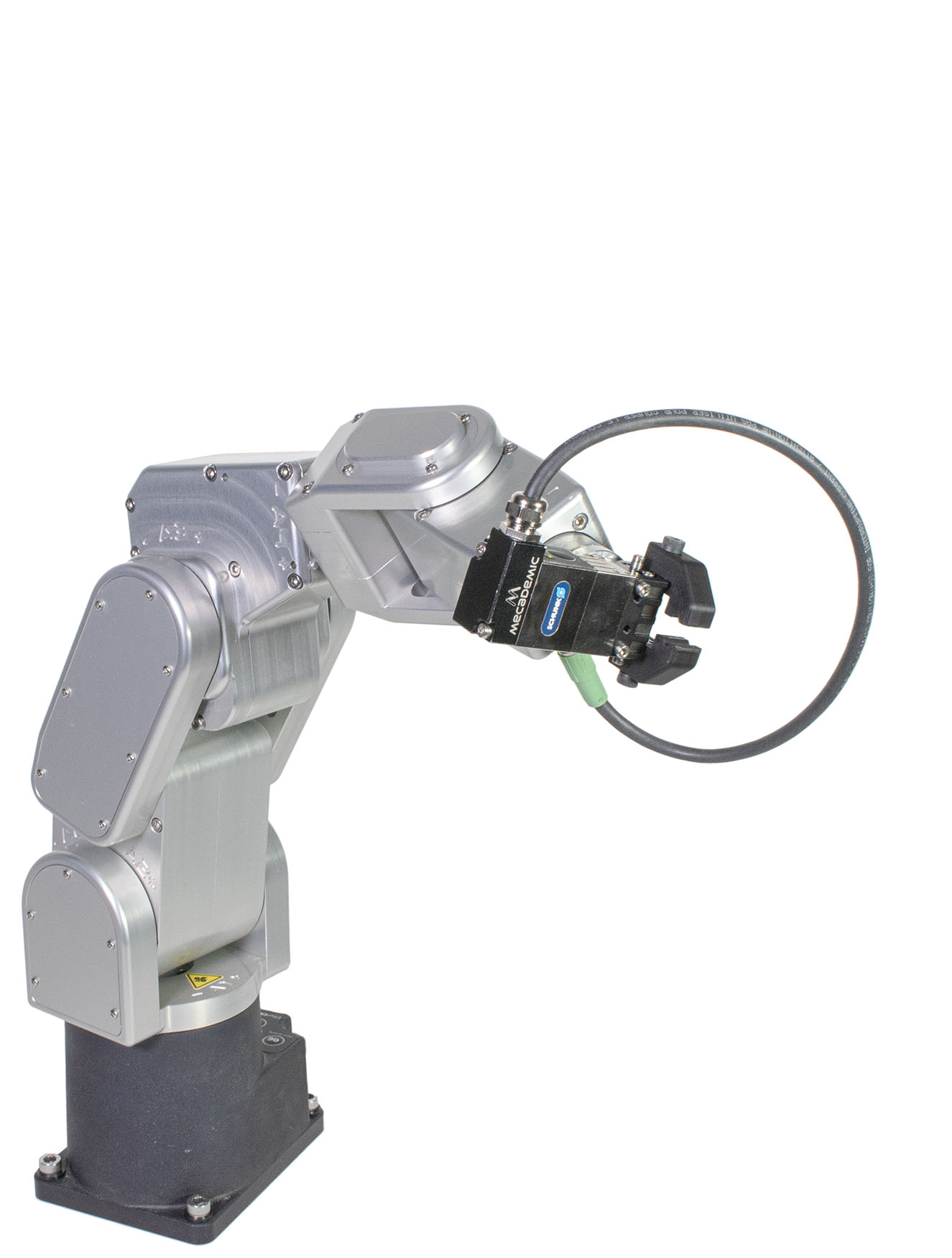
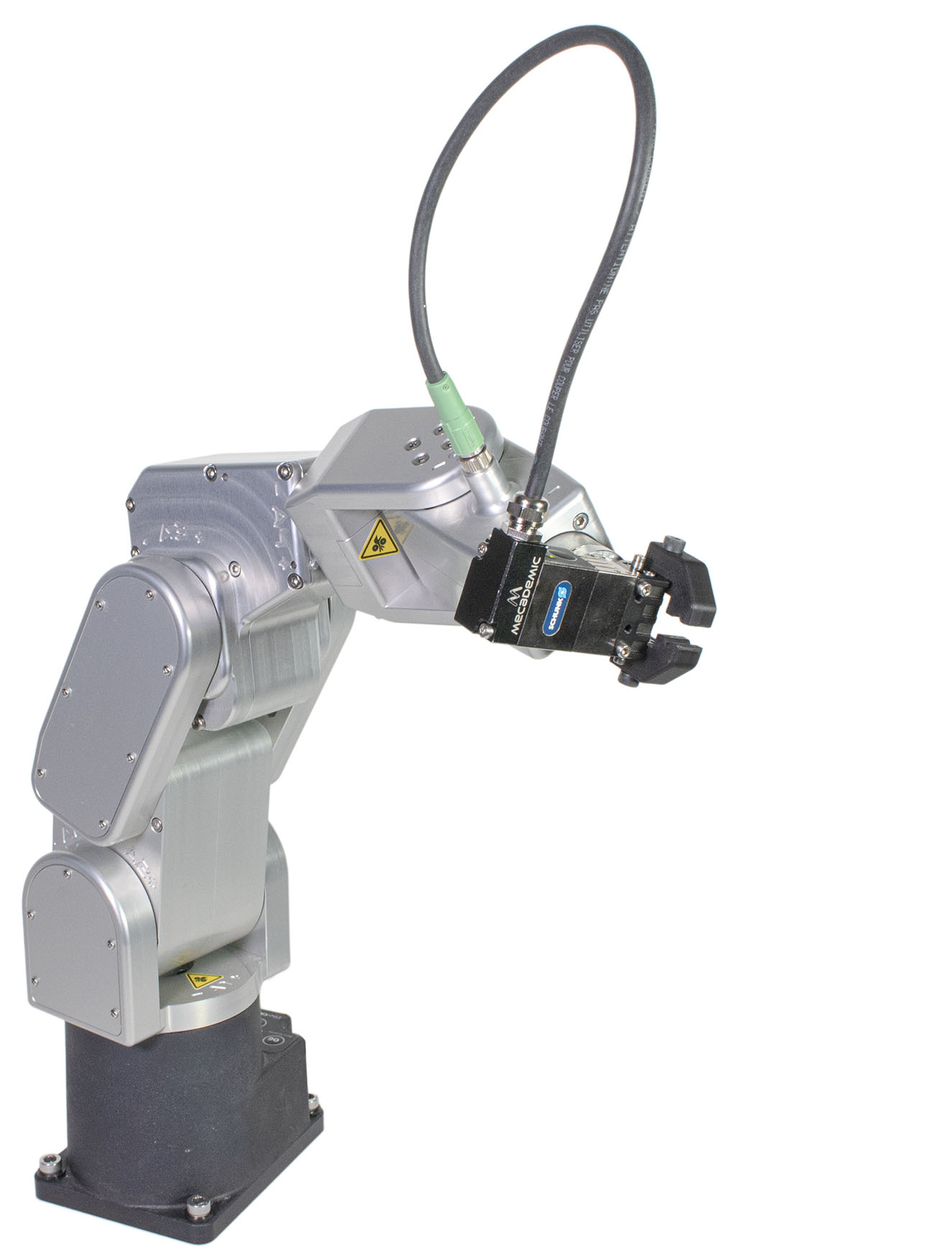
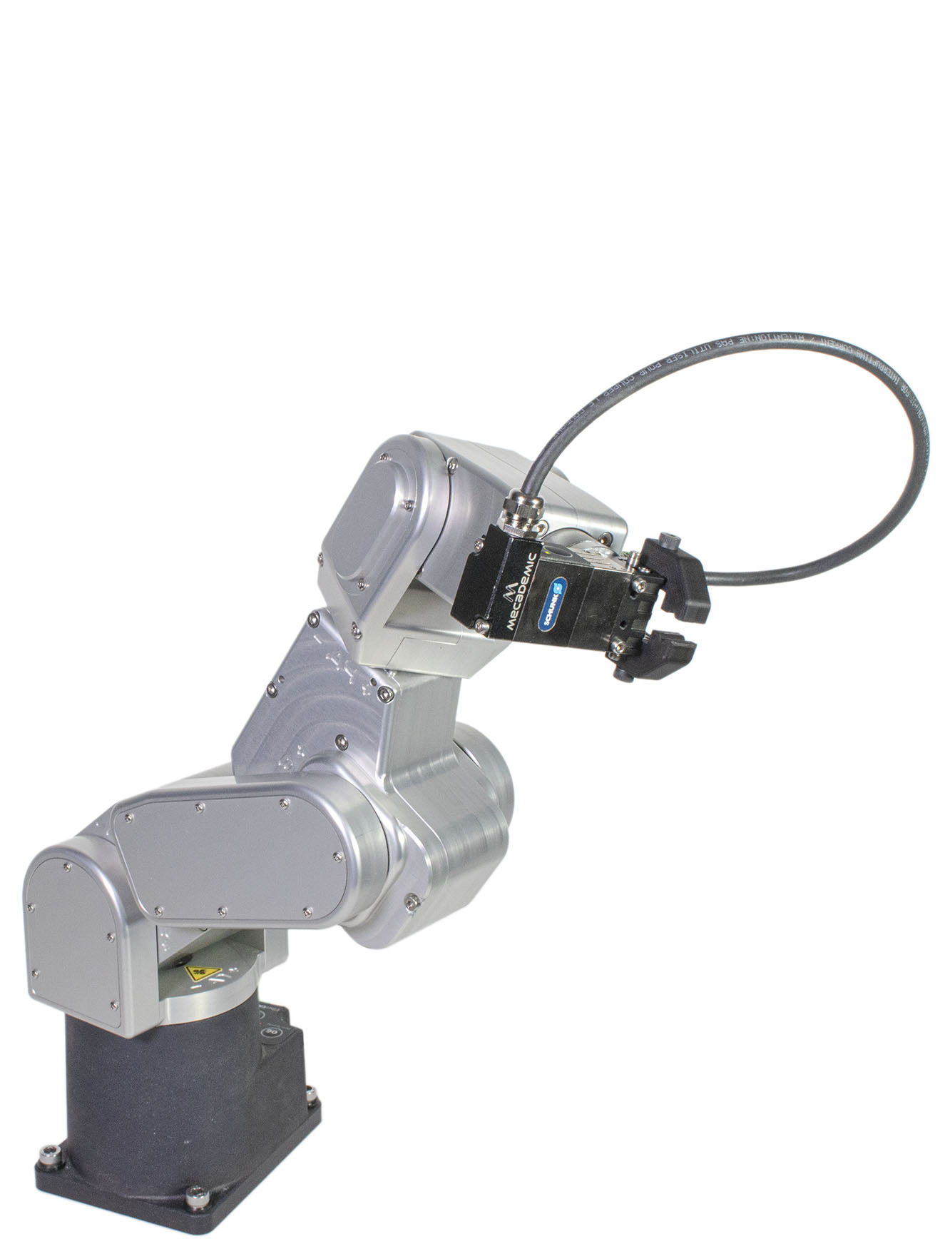
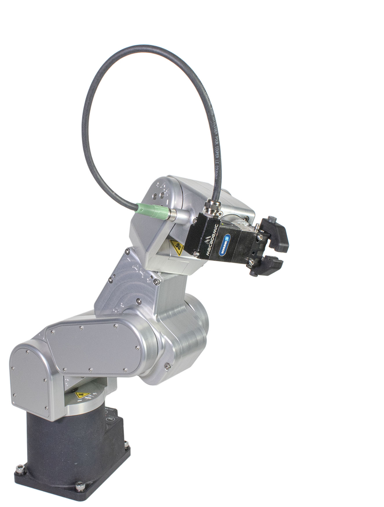
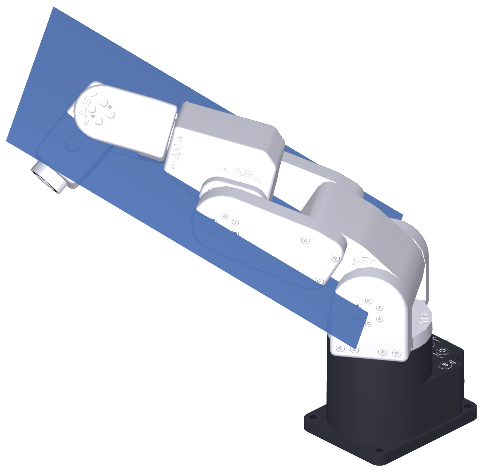
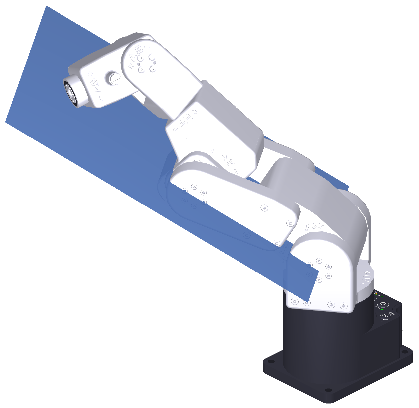
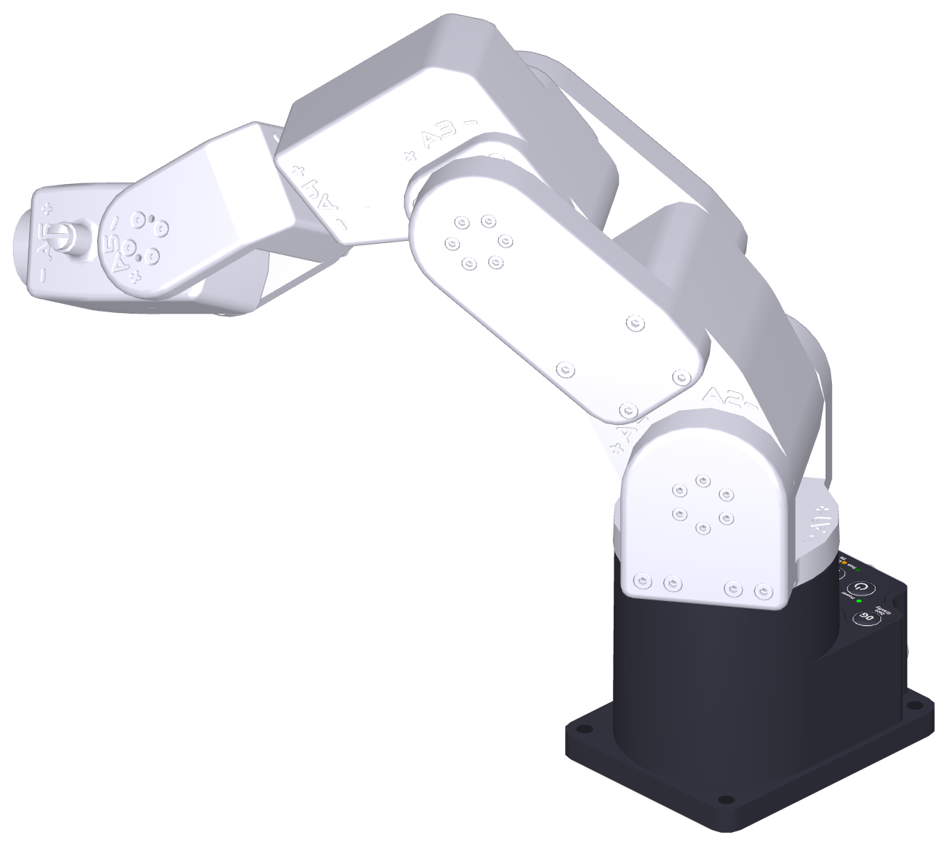
The joints of the Meca500 are numbered in ascending order, starting from the base, as shown in Figure 1a. Figure 1 also shows the zero joint positions. In that “zero” robot position, the axis of joint 3 intersects the axis of joint 1, the axes of joints 4 and 6 are aligned and normal to the axis of joint 1, and the axes of joints 2, 3, and 5 are parallel. Finally, note the location of the small screw in the robot’s flange, which is the 20-mm disk with threaded holes at the extremity of the robot arm.
 (a) robot with all joints numbered and at zero degrees
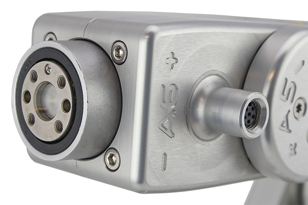 (b) robot's flange with joint 6 at zero degrees
 (a) robot with all joints numbered and at zero degrees
(b) robot's flange with joint 6 at zero degrees
(a) robot with all joints numbered and at zero degrees
(b) robot's flange with joint 6 at zero degrees
Figure 1 Meca500’s joint numbering and zero-degree joint position#
2.1.3. Reference frames#
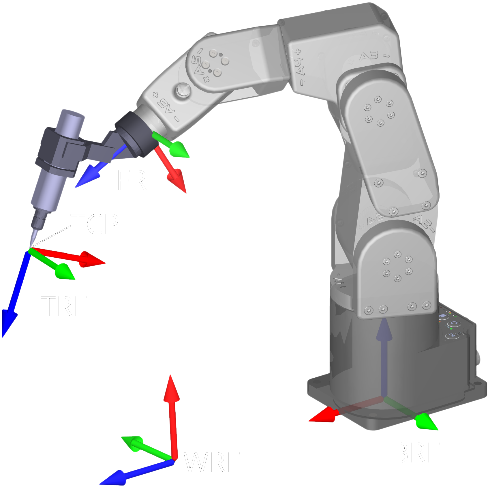
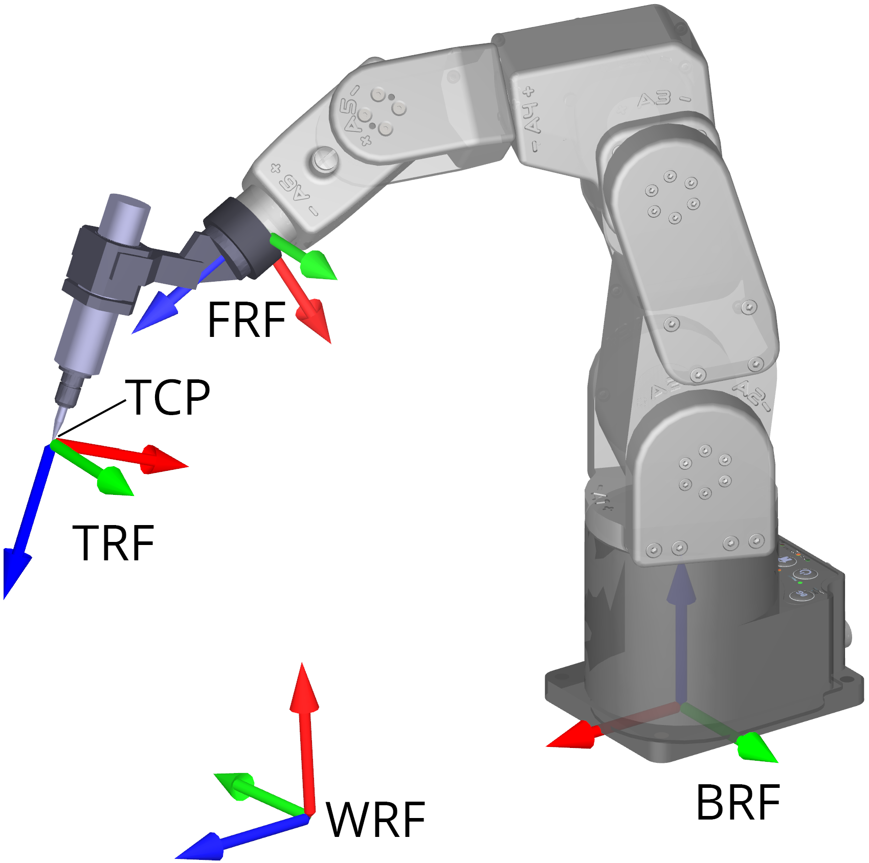
We use right-handed Cartesian coordinate systems (reference frames). There are only four of them that you need to be familiar with, as shown in Figure 2 (x axes are red, y axes are green, and z axes are blue). These four reference frames and the key term related to them are:
BRF: Base Reference Frame. Static reference frame fixed to the robot base. Its z axis coincides with the axis of joint 1 and points upwards, its origin lies on the bottom of the robot base, and its x axis is normal to the base front edge and points forward.
WRF: World Reference Frame. The main static reference frame coincides with the BRF by default. It can be defined with respect to the BRF using the
SetWrfcommand.
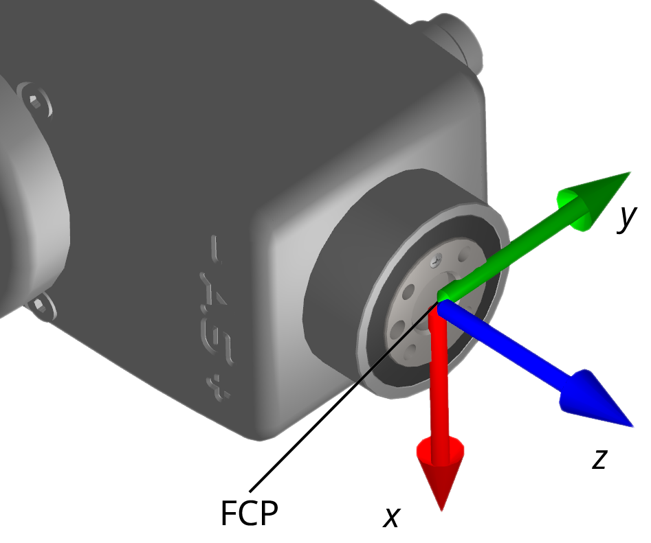
FRF: Flange Reference Frame. Mobile reference frame fixed to the robot’s flange. The z axis coincides with the axis of joint 6, and points outwards. Its origin lies on the plane passing through the flange’s mating surface. Finally, when all joints are at zero, the y axis of the FRF has the same direction as the y axis of the BRF.
FCP: Flange Center Point. Origin of the FRF.
TRF: Tool Reference Frame. The mobile reference frame associated with the robot’s end-effector. By default, the TRF coincides with the FRF. It can be defined with respect to the FRF with the
SetTrfcommand.TCP: Tool Center Point. Origin of the TRF. (Not to be confused with the Transmission Control Protocol acronym, which is also used in this document.)
 (a) All frames
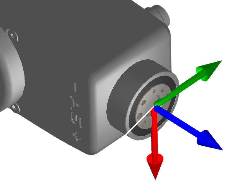 (b) Flange Reference Frame (FRF)
 (a) All frames
 (b) Flange Reference Frame (FRF)
Figure 2 Reference frames for the Meca500#
2.1.4. Pose and Euler angles#
Some Mecademic commands accept pose (position and orientation of one reference frame with respect to another) as arguments. In these commands, and in the MecaPortal web interface, a pose consists of a Cartesian position, {x, y, z}, and an orientation specified in Euler angles, {α, β, γ}, according to the mobile XYZ convention (also referred to as XYZ instrinsic rotations, RxRyRz, or XY’Z’’). In this convention, if the orientation of a frame F1 with respect to a frame F0 is described by the Euler angles {α, β, γ}, it means that if you align a frame Fm with frame F0, then rotate Fm about its x axis by α (alpha) degrees, then about its y axis by β (beta) degrees, and finally about its z axis by γ (gamma) degrees, the final orientation of frame Fm will be the same as that of frame F1.
Figure 3 shows an example of specifying orientation using the mobile XYZ Euler angle convention. The diagram on the right shows the black reference frame orientation with respect to the gray reference frame with the Euler angles {45°, −60°, 90°}.
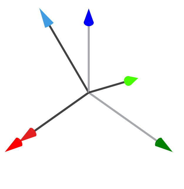 (a) rotate 45° about the x axis
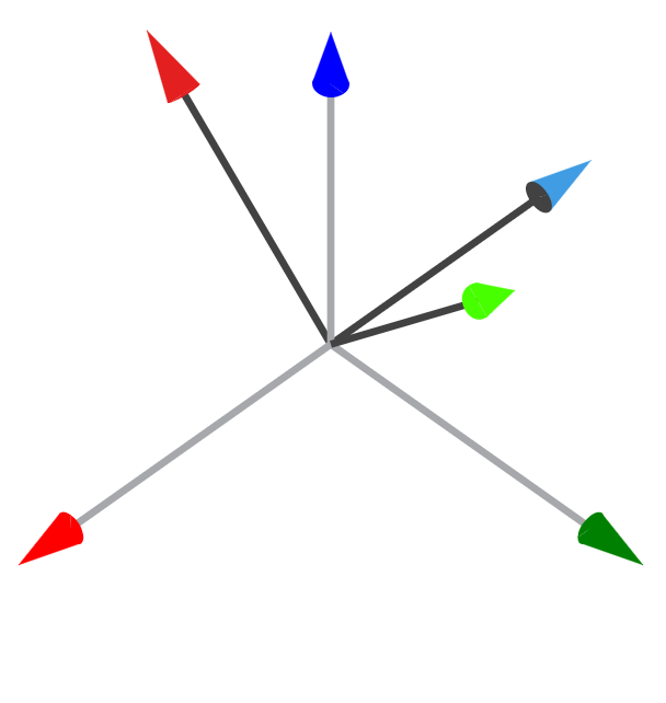 (b) rotate −60° about the new y axis
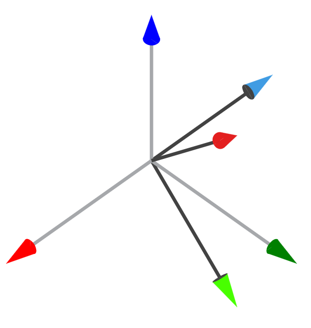 (c) rotate 90° about the new z axis
Figure 3 The three consecutive rotations associated with the Euler angles {45°, −60°, 90°}#
Because there are infinitely many sets of Euler angles that define a given orientation, the commands that accept a pose as arguments accept any numerical value for the three Euler angles (e.g., the set {378.34°, −567.32°, 745.03°}). However, we output only the equivalent Euler angle set {α, β, γ}, for which −180° ≤ α ≤ 180°, −90° ≤ β ≤ 90° and −180° ≤ γ ≤ 180°. Furthermore, if you specify the Euler angles {α, ±90°, γ}, the controller will always return an equivalent Euler angle set with α = 0. Thus, it is perfectly normal that the Euler angles used to specify an orientation are not the same as the Euler angles returned by the controller, once that orientation has been attained (see our tutorial on Euler angles).
Note
There are always at least two sets of Euler angles that define a given orientation — even when all angles are confined to the range ±180° — and in some cases, there are infinitely many. It is therefore possible that the controller returns a set of Euler angles that is different from the one you specified.
2.1.5. Joint positions and last joint turn configuration#
The angle associated with a rotational joint i, θi, will be referred to as joint position i. Since the last joint of the robot (joint 6) can rotate more than one revolution, the joint angle should be interpreted as a motor angle, rather than as the angle between two consecutive robot links. Unless you attach an end-effector with cabling to the robot flange, the value of the last joint angle cannot be determined by visual inspection alone.
Note that the directions of rotation for each joint are engraved on the robot’s body. As previously mentioned, all joint positions are zero in Figure 1.
The mechanical limits of the first five joints of the Meca500 are as follows:
Joint 6 has no mechanical limits, but its software limits are ±100 turns. Finally, we define the integer ct as the joint 6 turn configuration parameter, so that
Joints can be further constrained using the SetJointLimits command (or via
the MecaPortal).
2.1.6. Joint set and robot posture#
There are several possible solutions for joint positions, for a desired pose of the robot end-effector with respect to the robot base, i.e., several possible sets {θ1, θ2, θ3, θ4, θ5, θ6}. The simplest way to describe how the robot is postured, is by giving its set of joint positions. This set will be referred to as the joint set.
A joint set completely defines the relative poses of each pair of adjacent links, i.e., the robot posture. However, the joint sets {θ1, θ2, θ3, θ4, θ5, θ6} and {θ1, θ2, θ3, θ4, θ5, θ6 + ct 360°}, where −180° < θ6 ≤ 180° and ct is the turn configuration for joint 6, define the same robot posture.
Therefore, a joint set conveys the same information as a robot posture AND the turn configuration of the last joint.
2.2. Configurations, singularities and workspace#
2.2.1. Inverse kinematic solutions and configuration parameters#
Inverse kinematics is the problem of obtaining the robot joint sets that correspond to a desired end-effector pose.
 (a) {1, 1, 1}
 (b) {1, 1, −1}
 (c) {1, −1, 1}
 (d) {1, −1, −1}
 (e) {−1, 1, 1}
 (f) {−1, 1, −1}
 (g) {−1, −1, 1}
 (h) {−1, −1, −1}
Figure 4 An example showing all eight possible robot postures of the Meca500 for the same end-effector pose#
The inverse kinematics of our six-axis robots provide up to eight feasible robot postures for a desired pose of the TRF with respect to the WRF, as shown in Figure 4, and many more joint sets (since if θ6 is a solution, then θ6 ± m360°, where m is an integer, is also a solution). Each of these solutions is associated with a different combination of three parameters called the robot posture configuration parameters: cs, ce and cw. Each of these parameters corresponds to a specific geometric condition on the robot posture:
cs (shoulder configuration parameter)
cs = 1, if the wrist center (where the axes of joints 4, 5, and 6 intersect) is on the “front” side of the plane passing through the axes of joints 1 and 2 (see Figure 5a).
cs = −1, if the wrist center is on the “back” side of this plane (see Figure 5c).
ce (elbow configuration parameter)
cw (wrist configuration parameter)
Figure 4 shows an example with all eight possible robot postures, described by the posture configuration parameters {cs, ce, cw}, for the pose {77 mm, 210 mm, 300 mm, −103°, 36°, 175°} of the FRF with respect to the BRF.
Figure 5 shows an example of each robot posture configuration parameter, and limit conditions, which are called singularities. (We will discuss singularities in the next section.) Note that the popular terms front/back and elbow-up/elbow-down are misleading as they are not relative to the robot base but to specific planes that move when some of the robot joints rotate.
 (a) cₛ = 1, front
 (b) shoulder singularity
 (c) cₛ = −1, back
 (d) cₑ = 1, elbow up
 (e) elbow singularity
 (f) cₑ = −1, elbow down
 (g) cᵥᵥ = 1, noflip
 (h) wrist singularity
 (i) cᵥᵥ = −1, flip
Figure 5 Posture configuration parameters and the three singularity types for the Meca500#
The robot calculates the solution to the inverse kinematics that corresponds to the
desired posture configuration, {cs, ce, cw}, defined by
the SetConf command. In addition, it solves θ6 by choosing the
angle that corresponds to the desired turn configuration, ct, defined by the
SetConfTurn command. The turn is therefore the last inverse kinematics
configuration parameter.
Both the turn configuration and the set of robot posture configuration
parameters are needed to pinpoint the solution to the robot inverse kinematics
(i.e., to pinpoint the joint set corresponding to the desired pose). However, there
are major differences between the turn and robot posture configuration parameters;
mainly that the change of turn does not involve singularities. This is why different
commands are used (SetConf and SetConfTurn,
SetAutoConf and SetAutoConfTurn, etc.).
Although it is possible to calculate the optimal inverse kinematic solution (the
shortest move from the current robot position) using the commands SetAutoConf
and SetAutoConfTurn, we strongly recommend always specifying the desired
values for the configuration parameters with SetConf and
SetConfTurn. This should be done for every Cartesian-space command (e.g.,
MovePose and the various MoveLin* commands) when programming your
robot online (online programming).
If you are teaching the robot position and later want the end-effector to
move to the current pose along a linear path, you must record not only the current pose
of the TRF relative to the WRF (using GetRtCartPos), but also the definitions
of both the TRF and the WRF (using GetTrf and GetWrf).
Additionally, you need to capture the corresponding configuration parameters (using
GetRtConf and GetRtConfTurn). Then, to ensure accurate execution
of the command MoveLin when approaching the previously recorded robot
position from a starting position, you must verify that the robot is already in the same
posture configuration and that θ6 is within half a
revolution of the desired value. If you do not require the robot’s TCP to follow a
linear trajectory, it is preferable to retrieve only the current joint set using
GetRtJointPos. You can later move the robot to that joint set with the
MoveJoints command, eliminating the need to record or specify the four
configuration parameters and the definitions of the TRF and WRF.
2.2.2. Automatic configuration selection#
The automatic configuration selection should only be used once you understand how this selection is done, and mainly while programming and testing. For example, when jogging in Cartesian space with the MecaPortal, the automatic configuration selection is always enabled. Or, if a target pose is identified in real-time based on input from a sensor (e.g., a camera), enabling the automatic configuration selection will increase your chances of reaching that pose, and in the fastest way.


Figure 6 Effect of configuration parameters on robot movement commands#
Figure 6 illustrates how the automatic and manual configuration selections work, with the following five remarks:
Setting a desired posture or turn configuration (with
SetConforSetConfTurn, respectively) disables the automatic posture or turn configuration selection, respectively, which are both set by default. Conversely, enabling the automatic posture or turn configuration selection, withSetAutoConf(1)orSetAutoConfTurn(1), respectively, removes the desired posture or turn configuration, respectively. At any moment, ifSetAutoConf(0)orSetAutoConfTurn(0)is executed, the robot posture or turn configuration of the current robot position is set as the desired posture or turn configuration, respectively.The commands
MoveJoints,MoveJointsRel, andMoveJointsVelignore the automatic and manual configuration selections. Thus, the robot may end up in a posture or turn configuration different from the desired ones, if such were set. If you want to update the desired configurations with the current ones, simply execute the commandsSetAutoConf(0)orSetAutoConfTurn(0).The command
MovePoserespects any desired posture or turn configuration, as long as the desired pose is reachable. In contrast, if automatic posture and/or turn configuration selection is enabled,MovePosewill choose the joint set corresponding to the desired end-effector pose, that is fastest to reach and that satisfies the desired posture or turn configuration, if any.In the case of
MoveLin*commands, the desired posture and turn configurations will force the linear move to remain within the specified posture and turn configurations. This means that aMoveLinorMoveLinRel*command will be executed only if the posture and turn configurations of the initial and final robot positions are the same as the desired configurations. In the case ofMoveLinVel*, the robot will start to move only if the posture and turn configurations of the initial and final robot positions are the same as the desired configurations, and will stop if desired configuration parameter has to change.When automatic configuration selection is enabled, a
MoveLin*command may lead to changing the posture (if passing through a wrist or shoulder singularity) or turn configuration along the path.
Finally, note that there is currently no way of specifying only one of the posture
configuration parameters and leaving the choice of the others to the robot
controller. However, there is an indirect way to specify the elbow and wrist
configurations, though this can’t be done “on the fly”. Indeed, if you prefer to
always stick to one of the two possible wrist configurations in the Meca500, you can
simply limit the range of joint 5, to either positive or non-negative values, using
the command SetJointLimits. Similarly, you can fix the elbow configuration
parameter by setting the range of joint 3 to be always smaller or larger than
−arctan(60/19) ≈ −72.43°.
2.2.3. Workspace and singularities#
Users often oversimplify the workspace of a six-axis robot arm as a sphere with a radius equal to the robot’s reach (the maximum distance between the axis of joint 1 and the center of the robot’s wrist). However, the actual Cartesian workspace of a six-axis industrial robot is a six-dimensional entity, encompassing all attainable end-effector poses (refer to our tutorial on workspace, available on our main website). This means the workspace depends on the choice of the Tool Reference Frame (TRF).
Complicating matters further, as discussed in the preceding section, a given end-effector pose can generally correspond to eight distinct robot postures (see Figure 4). Thus, the Cartesian workspace of a six-axis robot is the union of eight workspace subsets, each corresponding to one of these postures. While these subsets share overlapping regions, there are also areas exclusive to a single subset — poses that are accessible in only one posture due to joint limits. To fully exploit the robot’s workspace, it is often necessary to transition between these subsets. These transitions involve singularities, which can pose challenges when the robot’s end-effector is required to follow a specific Cartesian path.
Every six-axis industrial robot arm encounters singularities (refer to our tutorial on singularities). However, a notable advantage of six-axis robots like ours is that the axes of the last three joints intersect at a single point — the center of the robot’s wrist. This design makes these singularities straightforward to describe geometrically (see Figure 5). As a result, determining whether a robot posture is near a singularity is significantly easier for our robots compared to other designs.
In a singular robot posture, some of the joint set solutions corresponding to the pose of the TRF may coincide, or there may be infinitely many joint sets. The problem with singularities is that at a singular robot posture, the robot’s end-effector cannot move in certain directions. This is a physical blockage, not a controller problem. Thus, singularities are one type of workspace boundary (the other type occurs when a joint is at its limit, or when two links interfere mechanically).
Take the Meca500, for example, at its zero robot posture (Figure 1). At this robot posture, the end-effector cannot be moved laterally (i.e., parallel to the y axis of the BRF); it is physically blocked. In order to move in that direction, it would need to rotate joints 4 and 6 a quarter of turn in opposite directions first. Thus, singularities are not some kind of purely mathematical problem. They represent actual physical limits.
There are three types of singular robot positions, and these correspond to the conditions under which the configuration parameters cs, ce, and cw are not defined. The most common singular robot posture is called a wrist singularity and occurs when θ5 = 0° (Figure 5h). In this singularity, joints 4 and 6 can rotate in opposite directions at equal velocities while the end-effector remains stationary. You will run into this singularity frequently. The second type of singularity is called an elbow singularity (Figure 5e). It occurs when the arm is fully stretched (i.e., when the wrist center is in one plane with the axes of joints 2 and 3). In the Meca500, this singularity occurs when θ3 = −arctan(60/19) ≈ −72.43°. You will run into this singularity when you try to reach poses that are too far from the robot base. The third type of singularity is called a shoulder singularity (Figure 5b). It occurs when the center of the robot’s wrist lies on the axis of joint 1. You will run into this singularity when you work too close to the axis of joint 1.
The following video illustrates the three types of singularities mentioned above:
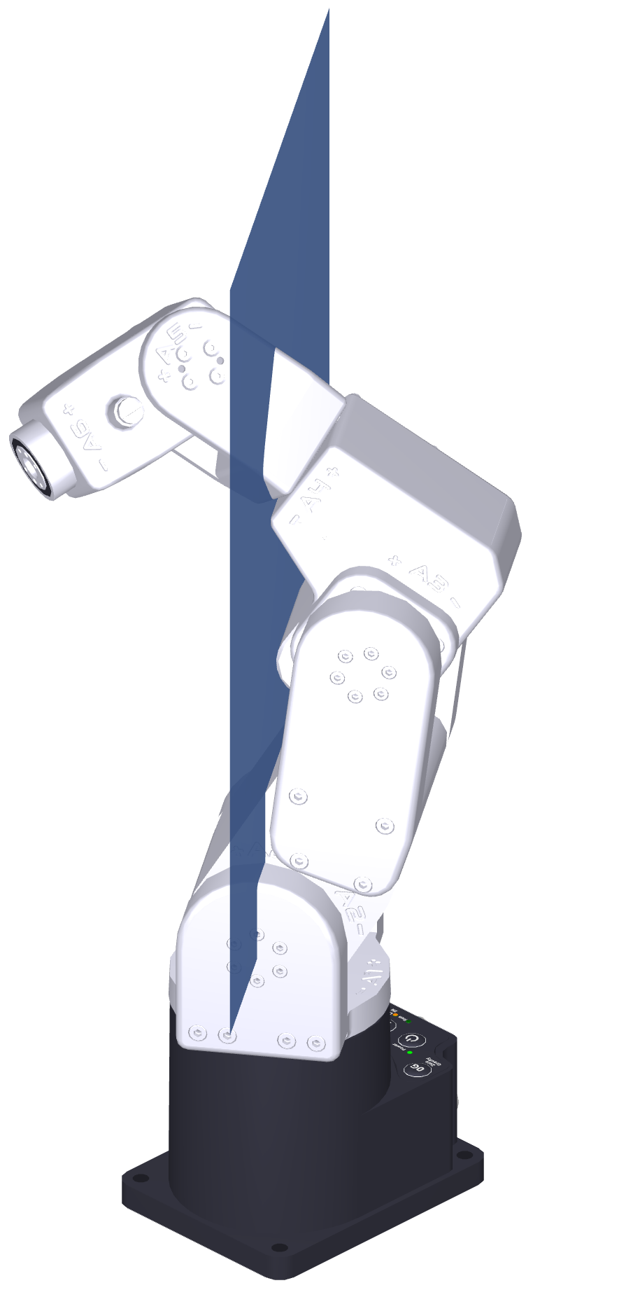
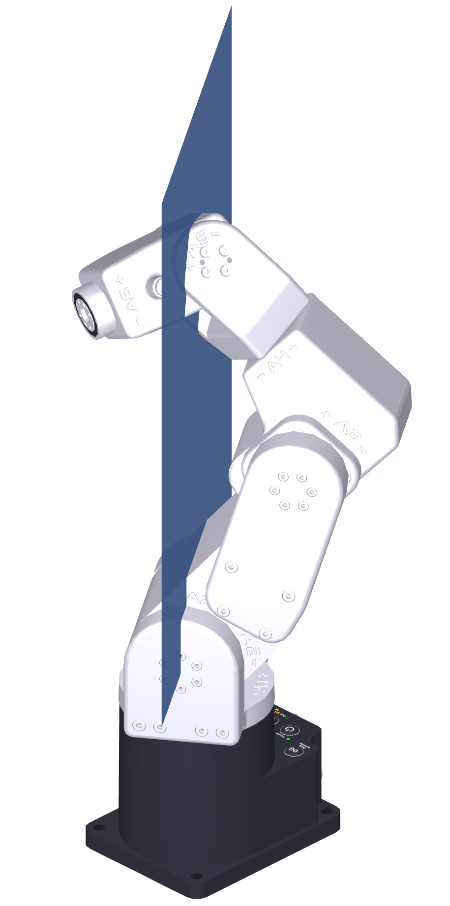
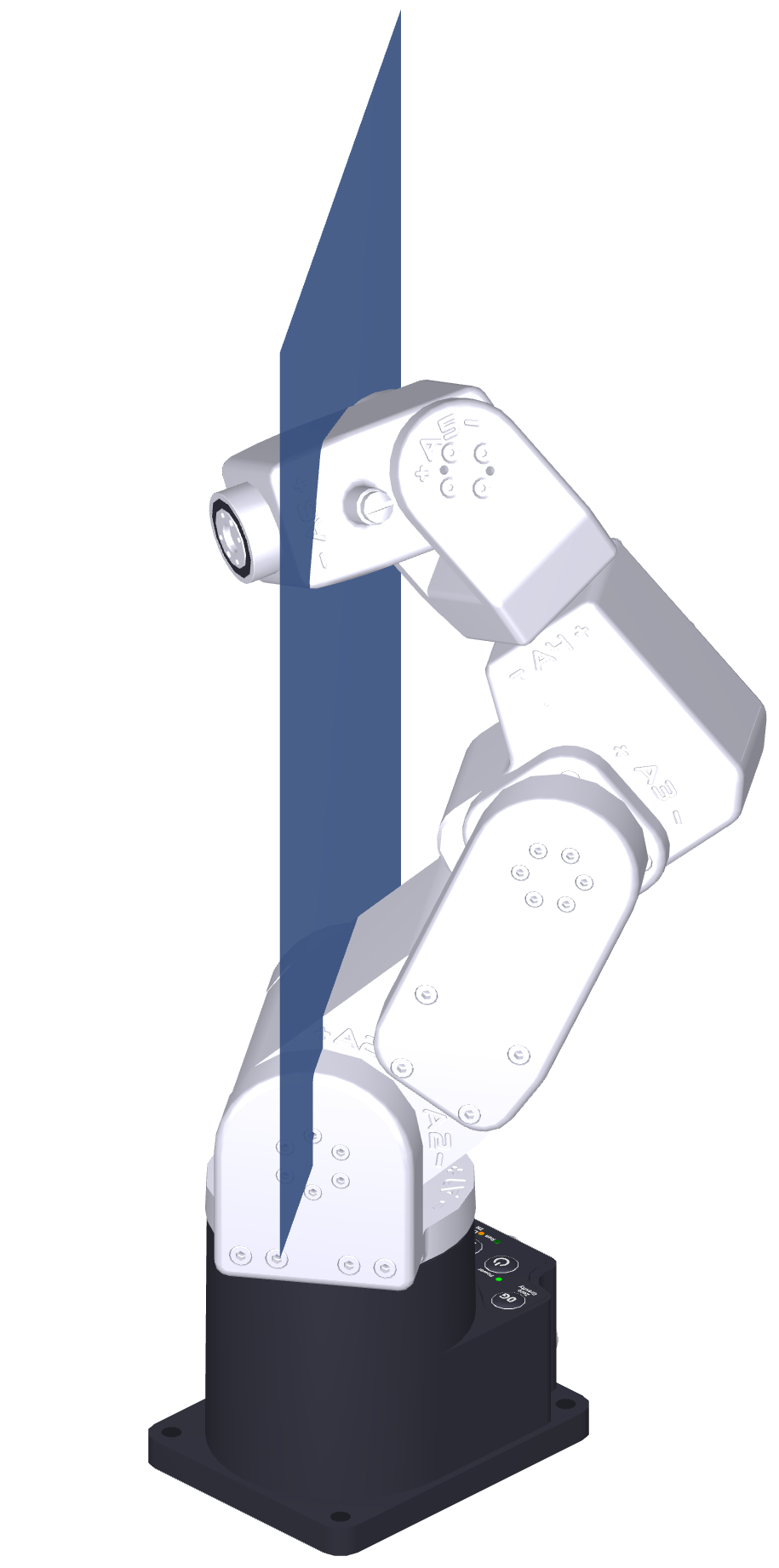
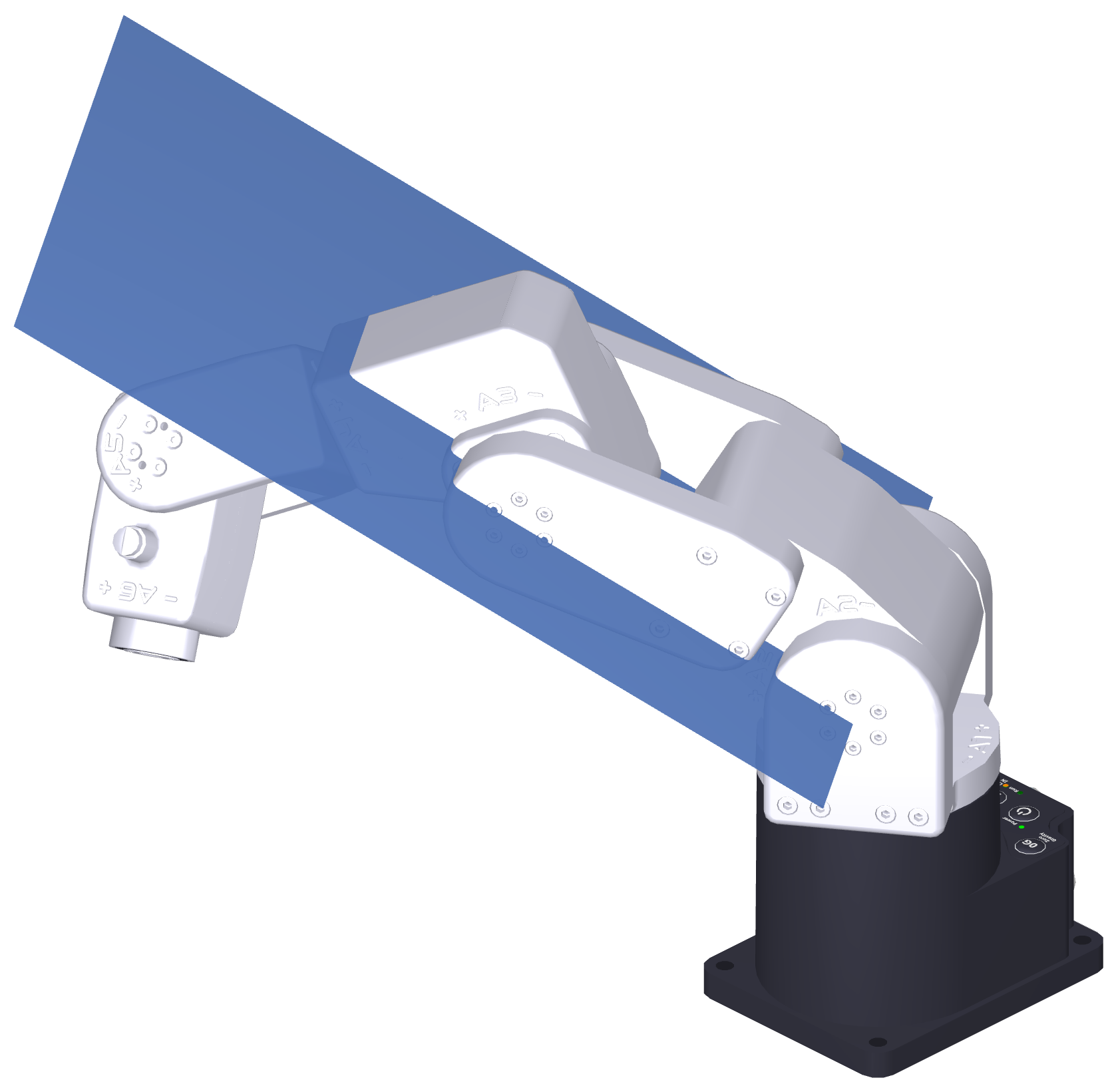
2.2.4. Crossing singularities with linear Cartesian-space movements#
Although singularities can be a nuisance when controlling the robot in
Cartesian space and should usually be avoided in production mode, we have made it
possible to cross them to facilitate programming our robots. With the release of
firmware 9.1, the Meca500 can start at or pass through wrist and shoulder
singularities, while executing any MoveLin* command, or end at any
singularity while executing a MoveLin* or MovePose command.
Furthermore, the passage respects the posture configuration selection settings
(Figure 6). Figure 7 illustrates how this feature makes
it possible to follow longer linear paths. In that figure, we start from an elbow
singularity, pass through a wrist singularity, then through a shoulder singularity,
and then end at another elbow singularity, all with a single MoveLin*
command, and in “AutoConf”.
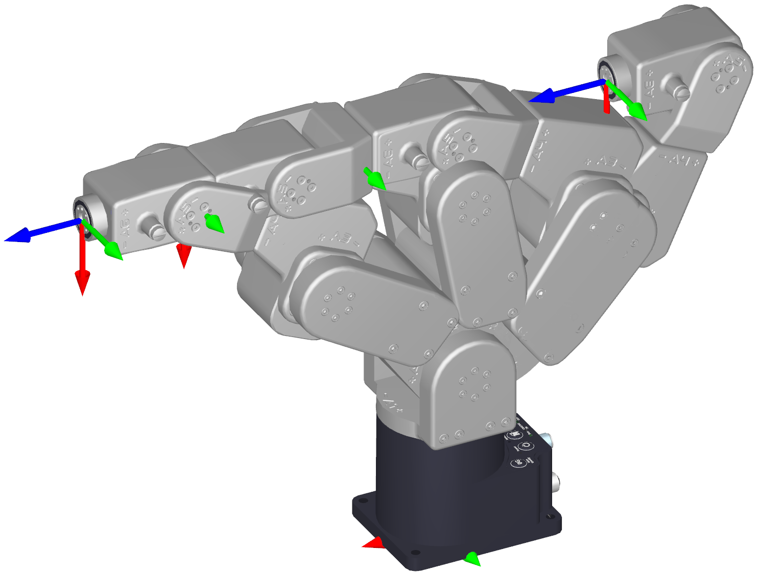
Figure 7 By crossing singularities, the Meca500 can execute longer linear movements#
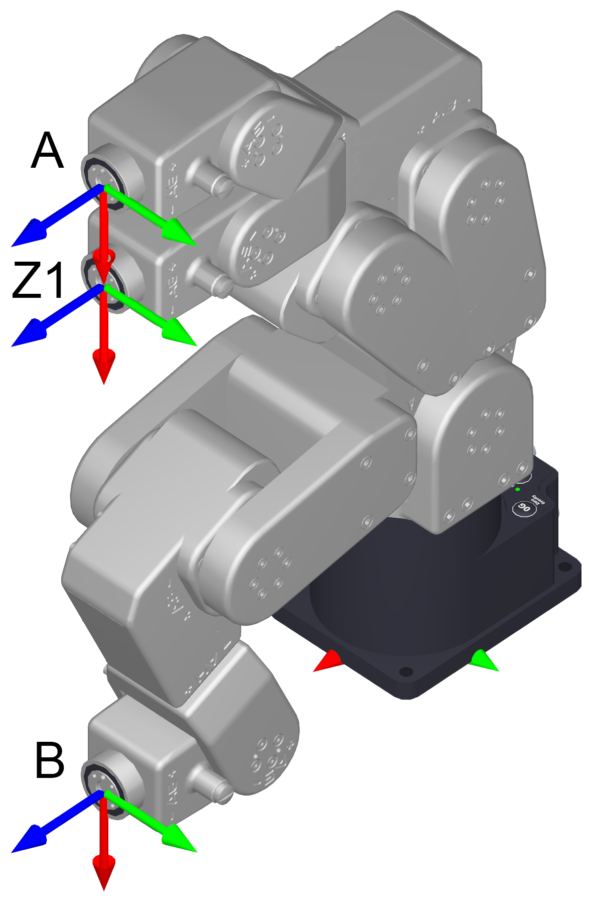
There are two possible situations when crossing a wrist singularity. Consider
Figure 8a, where “AutoConf” is enabled, the robot starts from robot
position A, passes without any interruption through the singular configuration Z1
(where all joints are at zero degrees) and goes to robot position B, all with a
single MoveLin* command. In the process, the robot changes the posture
parameter cw from 1 to −1. However, if you execute
SetConf(1,1,1), then request the robot to move with MoveLin*
to the end-effector pose B, starting from robot position A, the robot will refuse the
motion, since that would require joint 4 to rotate 180° or −180° when reaching robot
position Z1. This is impossible as the range of joint 4 is ±170°.
The following video illustrates the examples described above:
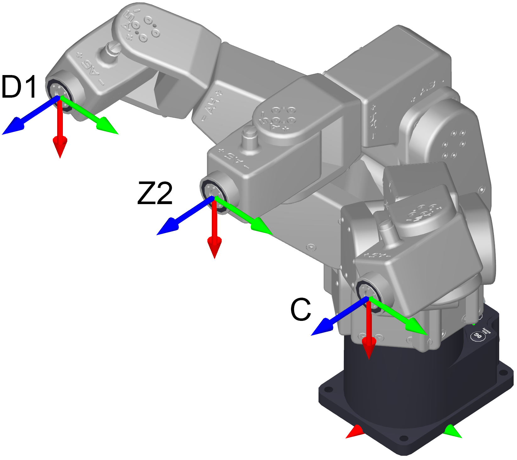
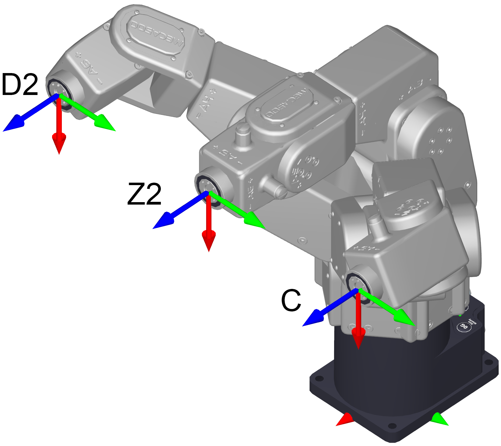
Similarly, consider Figure 8b, where “AutoConf” is enabled, the
robot starts from position C, passes without any interruption through the singular
configuration Z2 (where θ1 = θ2 = θ3 = θ5 = 0°,
θ4 = 90°, θ6 = −90°) and goes to robot position D1, all with a
single MoveLin command. In the process, the robot changes posture <
parameter cw from −1 to 1. However, as shown in Figure 8c,
if you execute SetConf(1,1,−1), then request the robot to move to the
end-effector pose D1, starting from robot position C, the robot will execute the
MoveLin command, but when it reaches configuration Z2, joint 4 will
rotate −180° and joint 6 will rotate 180°, at the same time while the end-effector
will remain stationary. After that, the robot will continue its linear motion and
reach the robot position D2 (which corresponds to the same pose as D1).
 (a) A↔B via Z1, only possible with AutoConf(1)
 (b) C↔D1 via Z2, when using AutoConf(1)
 (c) C↔D2 via Z2 and stationary re-orientation, with SetConf(1,1,−1)
Figure 8 Crossing a wrist singularity with SetAutoConf(1) or with a desired posture
configuration#
In contrast, since shoulder singularities are much less frequent, yet much more
complex to handle, the robot can currently cross them only in “AutoConf”. More
precisely, when executing a linear move, the robot will never stop at a shoulder
singularity to reorient its joints 1, 4 and 6 while keeping the end-effector
stationary. Thus, the motion sequence shown in Figure 9a cannot be
executed with a single MoveLin* command, whatever the state of posture
configuration selection. However, in “AutoConf”, you can cross a shoulder
singularity, as shown in Figure 9b. To experiment with shoulder
singularities, simply execute SetTrf(0,0,−70,0,0,0), to bring the TCP at
the wrist center, then SetWrf(0,0,0,0,0,0), and then bring the TCP to a
position where its coordinates x and y are zero.
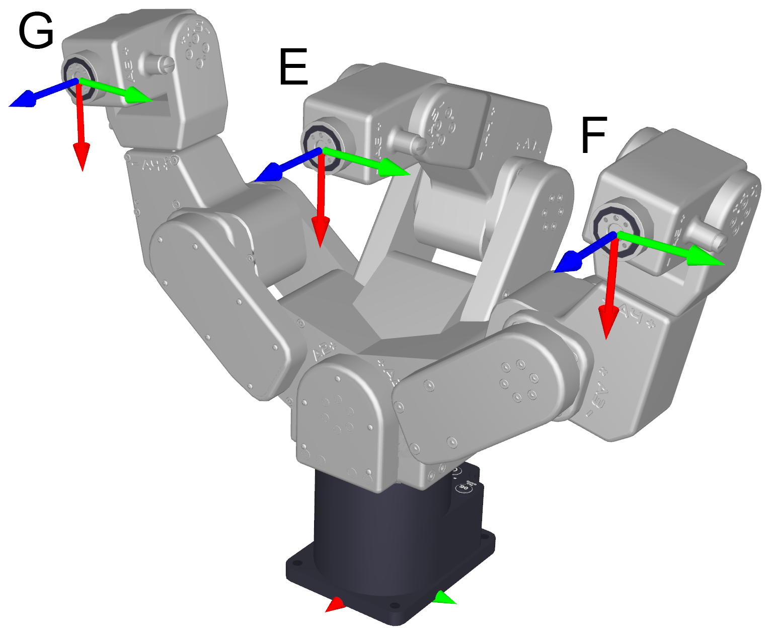 (a) Impossible sequence with a single MoveLin
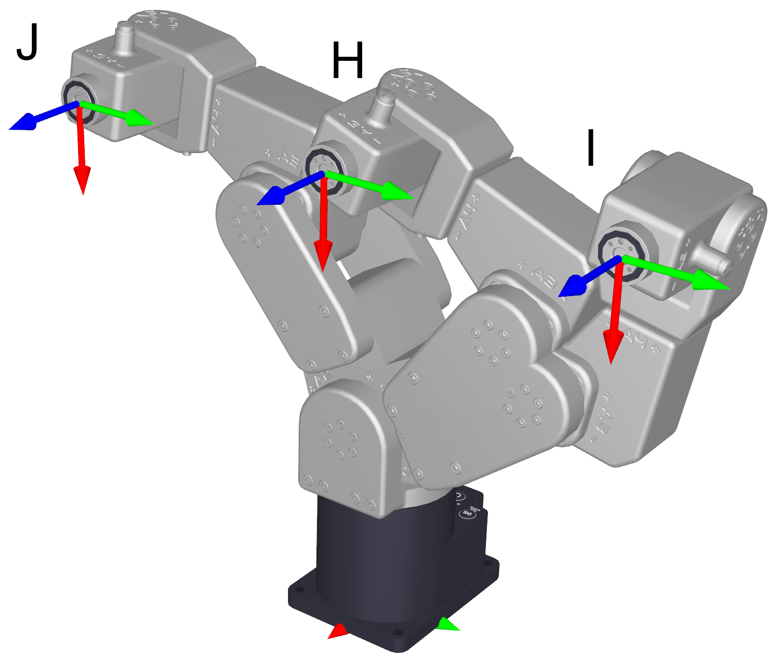 (b) I↔J via H, with AutoConf(1)
Figure 9 Crossing a shoulder singularity can only be done with SetAutoConf(1) and
implies a change of the posture parameter cs#
Passing exactly through singularities could be beneficial for some applications, but you must fully understand the concept. Otherwise, you might end up with highly suboptimal robot motions. For example, consider the motion shown in Figure 9b. If you try to follow the same linear path, but one micrometer closer to the z axis of the WRF, joints 4 and 6, or joints 1, 4 and 6, will rotate very fast while the end-effector’s speed will be significantly reduced, in a motion similar to what is shown in Figure 9a. Indeed, passing through or close to singularities often leads to longer cycle times, and should be avoided in production mode.
2.3. Key concepts for Mecademic robots#
2.3.1. Homing#
At power-up, the robot knows the approximate angle of each of its joints, with a couple of degrees of uncertainty. Each motor must make one full revolution to accurately find the exact joint angles. This motion is the essential part of a procedure called homing.
During homing, joints too close to a physical limit first rotate slightly away. Then,
all joints rotate simultaneously in the positive direction: 3.6° for joints 1, 2, and
3, 7.2° for joint 4, 10.8° for joint 5, and 12° for joint 6. Finally, they return to
their initial angles. The entire sequence lasts three seconds. Make sure there is
nothing that restricts these joint movements, or the homing process will fail.
Homing will also fail if any of the robot joints are outside their user-defined
limits (SetJointLimits), if the work zone has been breached
(SetWorkZoneLimits, SetWorkZoneCfg) or if a collision has been
software detected (SetCollisionCfg).
Finally, if your Meca500 is equipped with a MEGP 25* gripper, the robot controller will automatically detect it and home it in parallel with the robot joints, by fully opening, then fully closing the gripper. Make sure there is nothing that restricts the full range of motion of the gripper, except its fingers, while it is being homed.
Once the robot is homed, you do not need to home it again, even if you deactivate it,
and then reactivate it, unless you use the optional argument 1, i.e.,
ActivateRobot(1). In Meca500 R4, after an E-Stop has been reset, you do not
need to run the homing procedure again, unless the robot is equipped with an MEGP 25*
gripper (in that case, only the gripper is homed actually). If you call the homing
process, but homing was not needed, the robot will simply ignore the command (though
it will still respond with the [2002][Homing done.] message). If homing was needed
only for the MEGP 25* gripper, the gripper fingers will move, but not the robot.
Note
The range of the absolute encoder of joint 6 is only ±420°.
Therefore, you must always rotate joint 6 within that range before
deactivating the robot. Failure to do so may lead to an offset of ±120° in
joint 6. If this happens, unpower the robot and disconnect your tooling. Then,
power up and activate the robot, perform its homing, and zero joint 6. If the
screw on the robot’s flange is not as in Figure 1,
then rotate joint 6 to +720°, and deactivate the robot. Next, reactivate it with
the command ActivateRobot(1), which reinitializes the drives, then home
the robot, and zero joint 6 again. Repeat one more time if the problem is not
solved.
Note
Before homing is completed, the robot’s accuracy is lower than after homing. As a result:
The reported real-time position will be less accurate (
GetRtJointPos,GetRtJointVel,GetRtCartPos,GetRtCartVel, etc.);The robot may not reach the exact requested position when using Recovery mode to move the robot before homing.
2.3.2. Recovery mode#
If the robot is blocked by joint limits (SetJointLimits), work-zone limits
(SetWorkZoneLimits, SetWorkZoneCfg), collisions
(SetCollisionCfg), or proximity to obstacles, it may be necessary to move it
to a safe position (sometimes before performing homing).
For these situations, use the SetRecoveryMode command.
2.3.3. Blending#
Industrial robots are most often controlled in position mode, using two groups of commands:
With Cartesian-space commands (
MoveLin,MoveLinRelWrf,MoveLinRelTrf), the robot is instructed to move its end-effector towards a target pose along a specified Cartesian path. To follow a complex Cartesian path, it must be broken down into small linear segments and executed using multiple Cartesian-space commands. Recall that singularities can pose challenges when using Cartesian-space commands.With joint-space commands (
MoveJoints,MoveJointsRel,MovePose,MoveJump), the robot is instructed — directly or indirectly — to move its joints linearly towards a target joint set. Recall that when using joint-space commands, singularities are generally not an issue (except possibly for theMovePosecommand).
Often, the target poses or joint sets act as “via points,” where the goal is not to reach the target precisely but simply to pass near it. Blending enables the robot to transition smoothly between motion segments instead of stopping at the end of each segment and making sharp changes in direction. Blending can be thought of as taking a rounded shortcut.
Blending allows the trajectory planner to maintain the end-effector’s acceleration to a minimum between two position-mode joint-space movements or two position-mode Cartesian-space movements. When blending is activated, the trajectory planner will transition between the two paths using a blended curve (Figure 10). The higher the TCP speed, the more rounded the transition will be (the radius of the blending cannot be explicitly controlled, only the blending duration is configurable).


Figure 10 TCP path for two consecutive linear movements, with and without blending#
Even if blending is enabled, the robot will come to a full stop after a joint-space
movement that is followed by a Cartesian-space movement, or vice-versa. When blending
is disabled, each motion will begin from a full stop and end in a full stop. Blending
is enabled by default. It can be completely disabled or only partially enabled with the
SetBlending command.
Furthermore, if blending is enabled, the gripper motion commands
(MoveGripper, GripperOpen, GripperClose) will not
cause the robot to stop between two position-mode joint-space commands (blending will
occur normally). However, the gripper motion commands will force the robot to stop
when used between two position-mode Cartesian-space commands. Once the robot has
come to a stop, the gripper’s fingers will start moving at the same time as the
subsequent Cartesian-space movement. In contrast, the SetValveState
command will not cause the robot to stop. Blending will occur normally, and the
SetValveState command will be executed at the beginning of the blending
path.
2.4. Position and velocity modes#
As mentioned in the previous section, the conventional method for moving an industrial
robot involves either commanding its end-effector to reach a desired pose along a
specified Cartesian path or directing its joints to rotate to a desired joint set. This
basic control method is called position mode. If the robot needs to
follow a linear path, the Cartesian-space motion commands MoveLin,
MoveLinRelTrf, and MoveLinRelWrf should be used. To move the
robot’s end-effector to a specific pose (without concern for the path followed by the
end-effector) or to rotate the robot’s joints to a given joint set or by a specified
amount, the joint-space motion commands MovePose, MoveJoints, or
MoveJointsRel should be used, respectively.
In position mode, with Cartesian-space motion commands, it is possible to specify the
maximum linear and angular velocities, and the maximum accelerations for the
end-effector. Alternatively, you can specify the time duration of your movement.
However, you cannot set a limit on the joint accelerations. Thus, if the robot executes
a Cartesian-space motion command and passes very close to a singular robot posture, even
if its end-effector speed and accelerations are very small, some joints may rotate at
maximum speed (as defined by SetJointVelLimit) and with maximum acceleration.
Similarly, with joint-space motion commands, it is possible to specify the maximum
velocity and acceleration of the joints or the time duration of the movement. However,
it is impossible to limit either the velocity or the acceleration of the robot’s
end-effector. Figure 11 summarizes the possible settings for the
velocity and acceleration in position mode.
As mentioned, in position mode, you can specify either the desired velocities
(SetJointVel or SetCartLinVel and SetCartAngVel) or the
movement’s time duration (SetMoveDuration). This choice is made using the
SetMoveMode command. In velocity-based position mode, the robot
attempts to follow the specified velocities without exceeding them while respecting
acceleration limits. However, portions of the movement may not maintain the exact
desired velocities, and the robot will not notify you of these deviations. In
time-based position mode, you can use SetMoveDurationCfg to
define how the robot should respond if it cannot complete the movement within the
specified duration.
There is a second method to control a Mecademic robot, by defining either its end-effector velocity or its joint velocities. This robot control method is called the velocity mode. Velocity mode is designed for advanced applications such as force control, dynamic path corrections, or telemanipulation (for example, the jogging feature in the MecaPortal is implemented using velocity-mode commands).
Controlling the robot in velocity mode requires one of the three velocity-mode motion
commands: MoveJointsVel, MoveLinVelTrf or
MoveLinVelWrf. Note that the effect from a velocity-mode motion command
lasts the time specified in the SetVelTimeout command or until a new
velocity-mode command is received. This timeout must be very small (the default value
is 0.05 s, and the maximum value 1 s). For the robot to continue moving after this
timeout, another velocity-mode command can be sent before this timeout. This new
command will immediately replace the previous command and restart the timeout.
Position-mode and velocity-mode motion commands can be sent to the robot, in any order.
However, if the robot is moving in velocity mode, the only commands that will be
executed immediately, rather than after the velocity timeout, are other velocity-mode
motion commands and SetCheckpoint, GripperOpen and
GripperClose commands.
Note
There is a significant difference in the behavior of position- and velocity-mode motion commands. In position mode, if a Cartesian-space motion command cannot be completely performed due to a singularity or a joint limit, the motion will normally not start and a motion error will be raised, that must be reset.
In velocity mode, if the robot runs into a singularity that cannot be crossed or a
joint limit, it will simply stop without raising an error. Furthermore, the velocity
of the robot’s end-effector or of the robot joints is directly controlled, but is
subject to the constraint set by the SetJointVelLimit command. The
SetJointVelLimit command affects the position-mode commands too.
See Figure 11 for a complete description of how velocity and
acceleration settings affect the two modes.
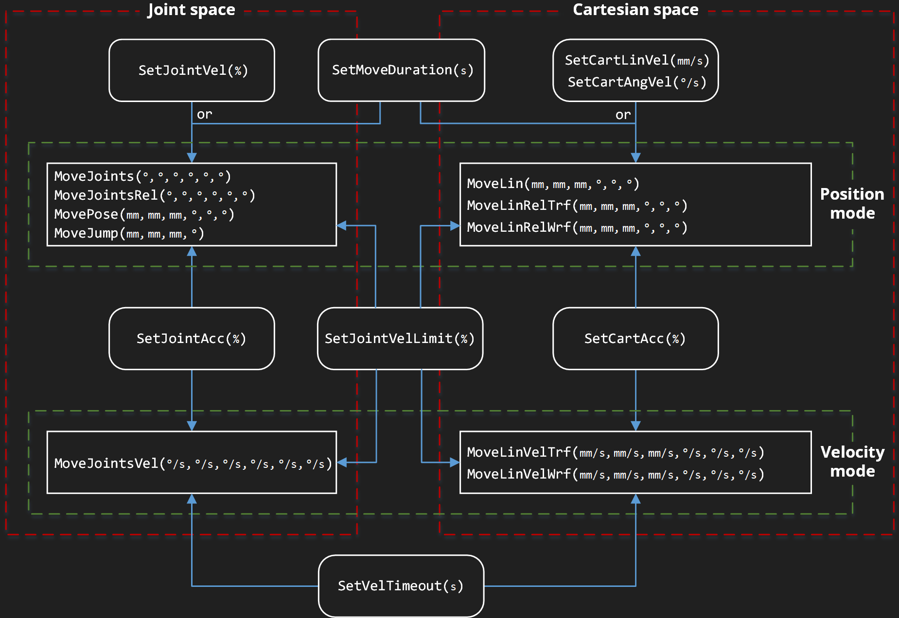
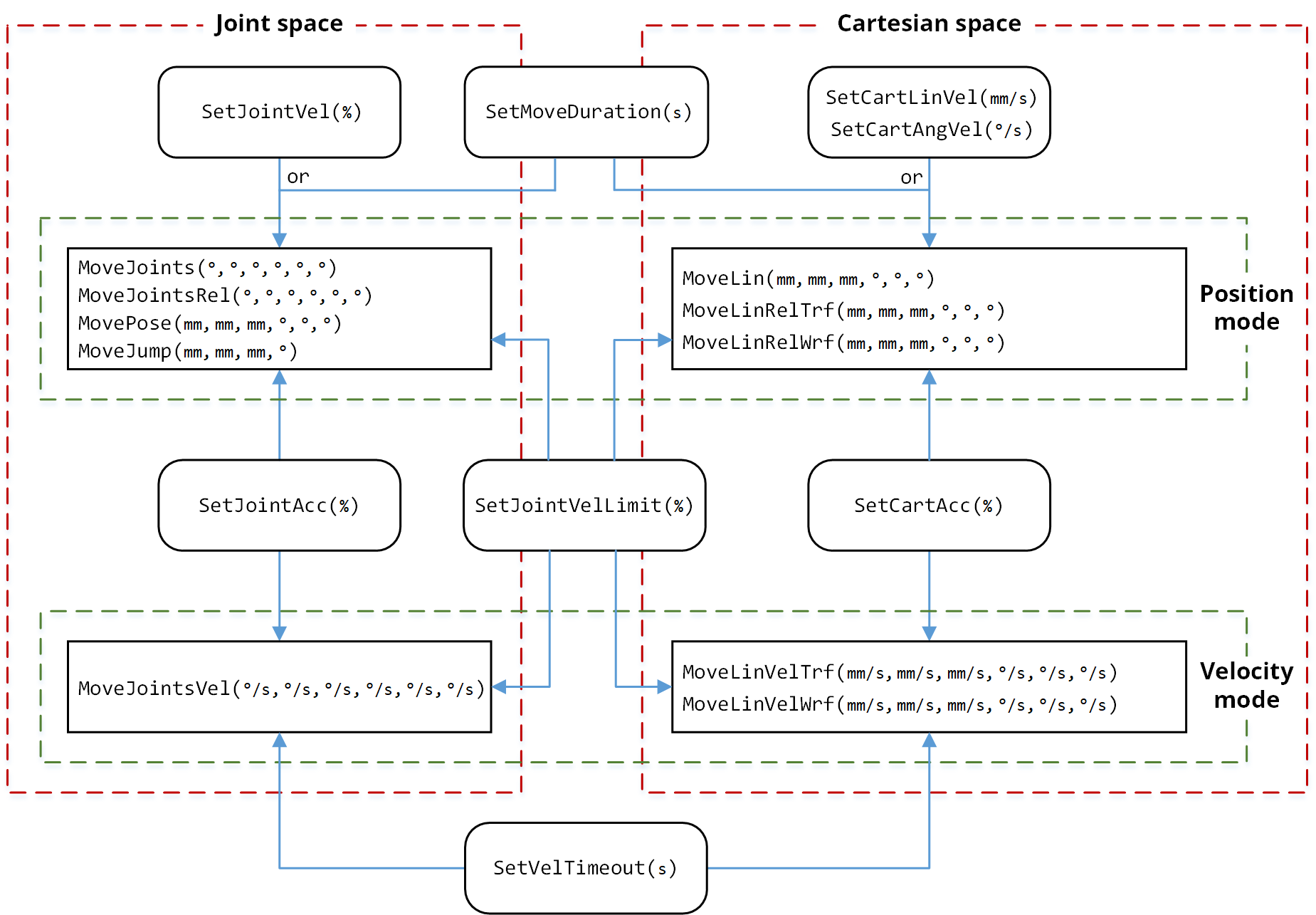
Figure 11 Settings that influence the robot motion in position and velocity modes.
Note that MoveJump is not supported and must not be used in time-based mode.#
Note
The instantaneous command SetTimeScaling affects all velocities,
accelerations and even time durations (including the timeout set with
SetVelTimeout and the pause set with the Delay command).