2. Basic theory and definitions#

We place a high value on technical accuracy, detail, and consistency, and use terminology that may not always align with standard industry terms. Therefore, it is important to read this section carefully, even if you have prior experience with industrial robot arms.

2.1. Definitions and conventions#

2.1.1. Units#

Distances that are displaced to or defined by the user are in millimeters (mm), angles are in degrees (°) and time is in seconds (s), except for timestamps.

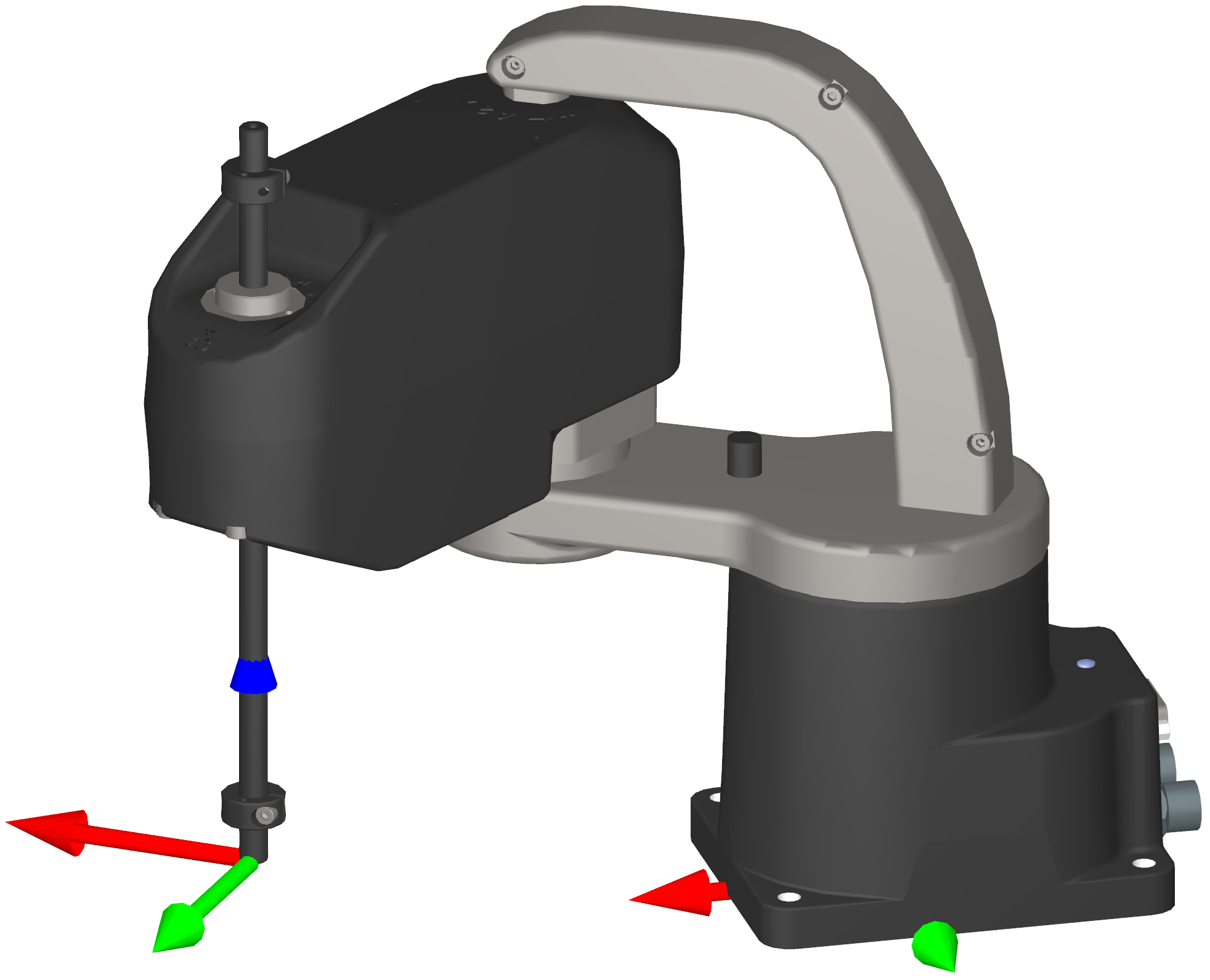
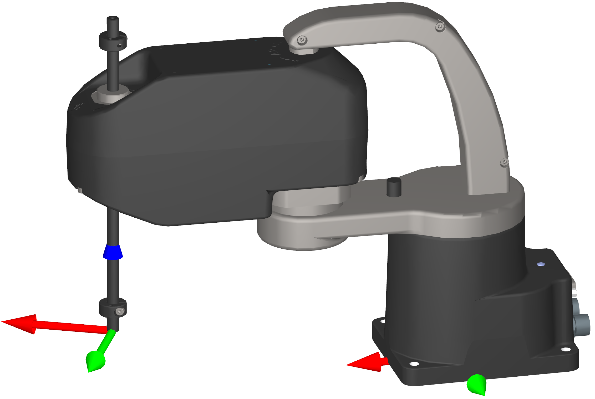
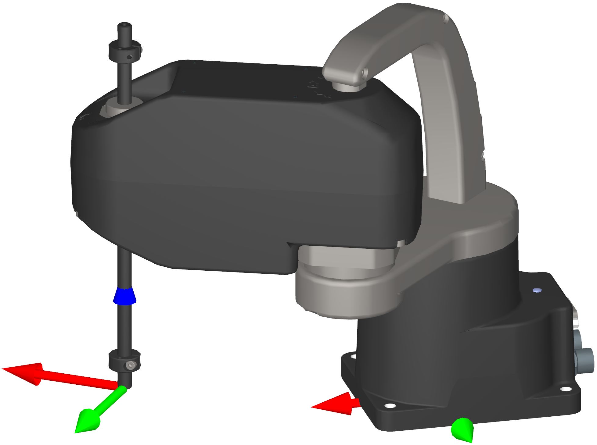
2.1.2. Joint numbering#

The joints of the MCS500 are also numbered in ascending order, starting from the base, but the last two “joints” are actually independent degrees of freedom, a translation and a rotation, and are achieved by driving a ball nut and a spline nut about a ball-screw spline. Thus, the translational motion is arbitrarily designated as joint 3, while the rotation about the spline shaft axis is designated as joint 4. Figure 1 shows the joint numbering, the joint directions and the zero joint position in the MCS500 robot. In that “zero” robot position, the axes of joints 1, 2, and 4 are coplanar and the spline shaft is all the way up.

MCS500's joint numbering, joint directions, and zero joint positions

2.1.3. Reference frames#

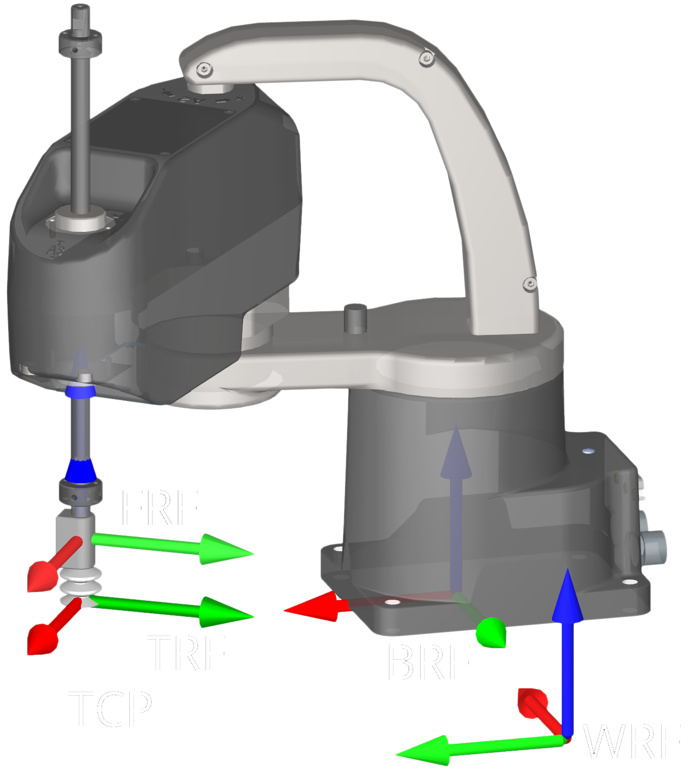
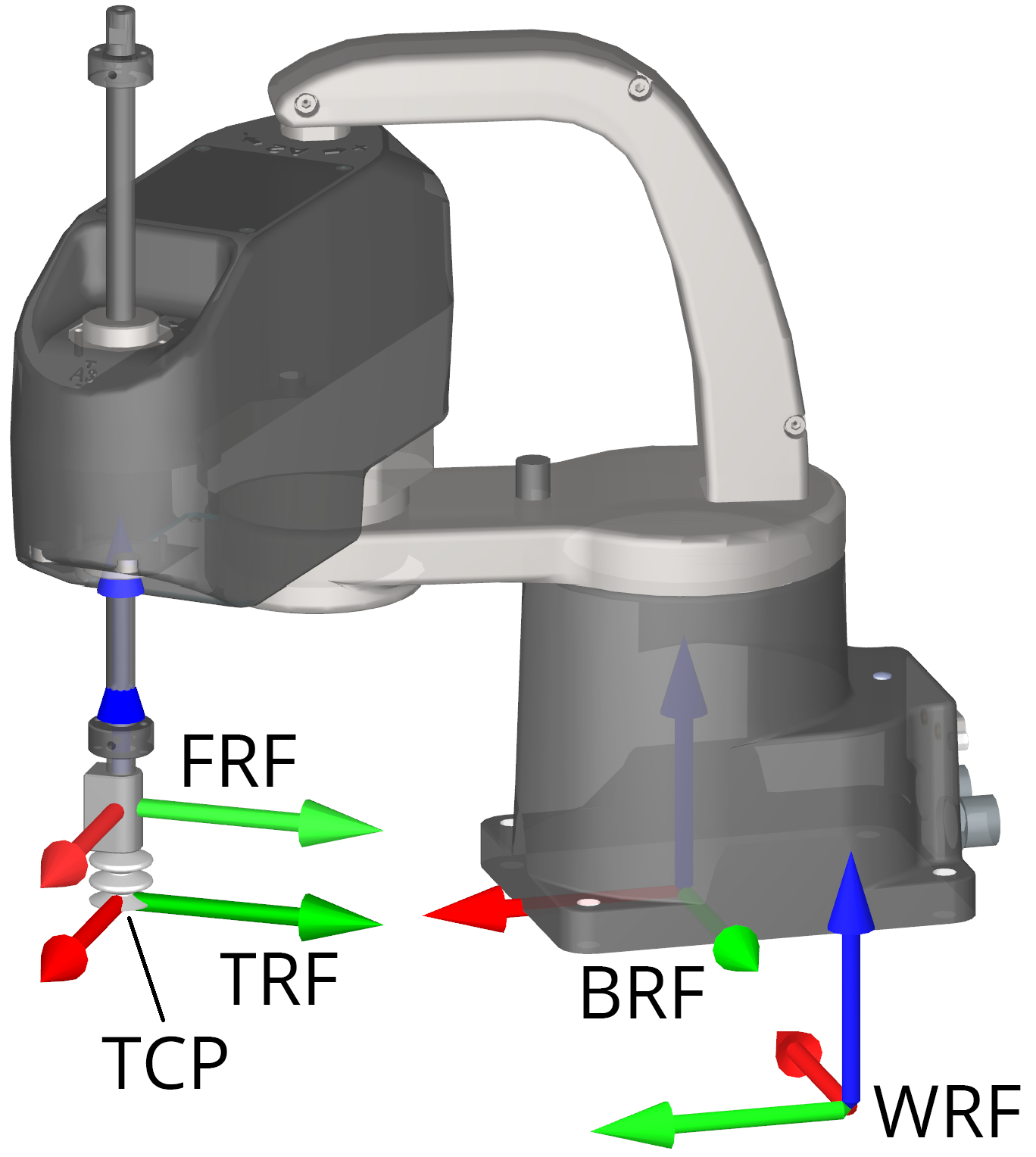
We use right-handed Cartesian coordinate systems (reference frames). There are only four of them that you need to be familiar with, as shown in Figure 2 (x axes are red, y axes are green, and z axes are blue). These four reference frames and the key term related to them are:

BRF: Base Reference Frame. Static reference frame fixed to the robot base. Its z axis coincides with the axis of joint 1 and points upwards, its origin lies on the bottom of the robot base, and its x axis is normal to the base front edge and points forward.
WRF: World Reference Frame. The main static reference frame coincides with the BRF by default. It can be defined with respect to the BRF using the SetWrf command.

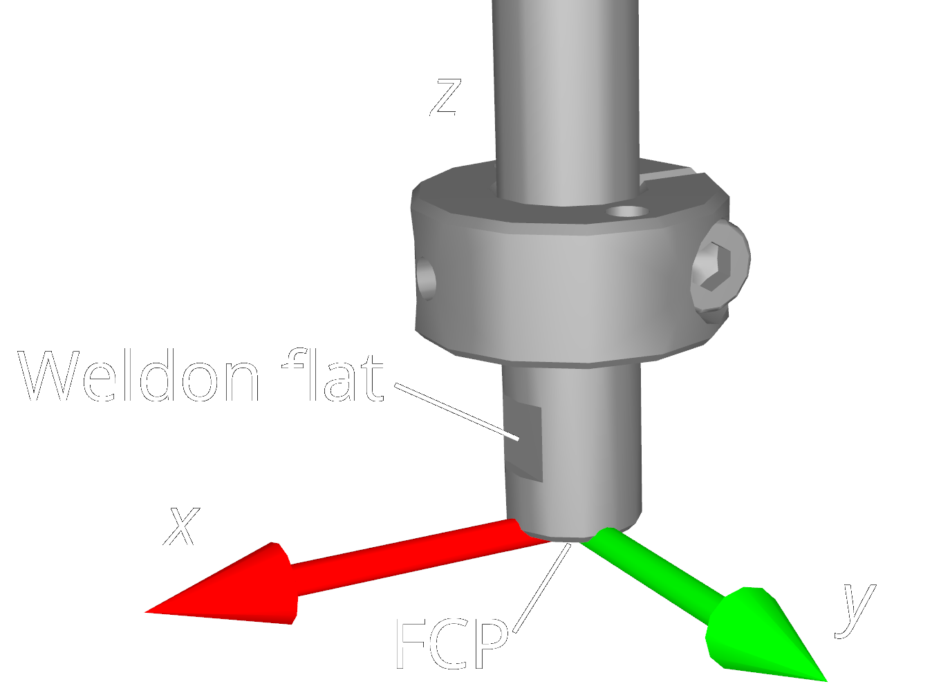
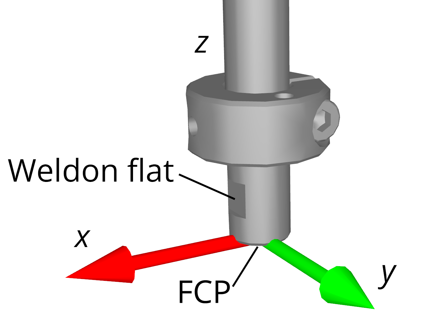
FRF: Flange Reference Frame. Mobile reference frame fixed to the robot’s flange. The FRF is fixed to the end of the spline shaft that is closer to the robot’s base, so that its z axis coincides with the axis of the spline shaft and points away from the robot’s base, its origin is at the very end of the spline shaft, and its x axis is perpendicular to the plane of the Weldon flat.

FCP: Flange Center Point. Origin of the FRF.
TRF: Tool Reference Frame. The mobile reference frame associated with the robot’s end-effector. By default, the TRF coincides with the FRF. It can be defined with respect to the FRF with the SetTrf command.
TCP: Tool Center Point. Origin of the TRF. (Not to be confused with the Transmission Control Protocol acronym, which is also used in this document.)

2.1.4. Pose#

Some Mecademic commands accept pose (position and orientation of one reference frame with respect to another) as arguments. In these commands, and in the the MecaPortal web interface, a pose consists of a Cartesian position, {x, y, z}, and the single orientation angle γ, about a vertical axis. All reference frames have their z axes upwards. It is impossible, for example, to specify a TRF with the z-axis pointing downwards.

2.1.5. Joint positions and last joint turn configuration#

The angle associated with the rotational joints 1, 2, and 4, θ₁, θ₂, and θ₄, respectively, and the position of the translational joint 3, d₃, will collectively be referred to as joint position i (i = 1, 2, 3, 4). Since the last joint of the robot (joint 4) can rotate more than one revolution, you should think of the joint angle as a motor angle, rather than as the angle between two consecutive robot links. Unless you attach an end-effector with cabling to the robot flange, there is no way of knowing the value of the last joint angle just by observing the robot.

Note that the directions for each joint are engraved on the robot’s body and shown in Figure 1. Also, as previously mentioned, all joint positions are zero in that figure.

The mechanical limits for the first three robot joints are as follows:

−140° ≤ θ1 ≤ 140°,
−145° ≤ θ2 ≤ 145°,
−102 mm ≤ d3 ≤ 0 mm.

Joint 4 has no mechanical limits, but its software limits are ±10 turns. Finally, we define the integer c_t as the joint 4 turn configuration parameter, so that

−180° + c_t360° < θ₄ ≤ 180° + c_t360°.

Joints can be further constrained using the SetJointLimits command (or via the MecaPortal).

2.1.6. Joint set and robot posture#

There are several possible solutions for joint positions, for a desired pose of the robot end-effector with respect to the robot base, i.e., several possible sets {θ₁, θ₂, d₃, θ₄}. The simplest way to describe how the robot is postured, is by giving its set of joint positions. This set will be referred to as the joint set.

A joint set completely defines the relative poses of each pair of adjacent links, i.e., the robot posture. However, the joint sets {θ₁, θ₂, d₃, θ₄} and {θ₁, θ₂, d₃, θ₄ + c_t 360°}, where −180° < θ₄ ≤ 180° and c_t is the turn configuration for joint 4, correspond to the same robot posture.

Therefore, a joint set conveys the same information as a robot posture AND the turn configuration of the last joint.

2.2. Configurations, singularities and workspace#

2.2.1. Inverse kinematic solutions and configuration parameters#

Inverse kinematics is the problem of obtaining the robot joint sets that correspond to a desired end-effector pose.

The inverse kinematics of our SCARA robots provide two feasible robot postures for a desired pose of the TRF with respect to the WRF, as shown in Figure 3, and many more joint sets (since if θ₄ is a solution, then θ₄ ± n360°, where n is an integer, is also a solution). These two solutions are distinguished with a parameter called the robot posture configuration parameter:

c_e (also called the elbow configuration parameter)
- c_e = 1, if θ₂ > 0°. The condition c_e = 1 is also referred to as “righty” (see Figure 3a);
- c_e = −1, if θ₂ < 0°. The condition c_e = −1 is also referred to as “lefty” (see Figure 3b);

(a) cₑ = 1, righty — Figure 3 Posture configuration parameter and the singularity in the MCS500#

(b) elbow singularity — Figure 3 Posture configuration parameter and the singularity in the MCS500#

The robot calculates the solution to the inverse kinematics that corresponds to the desired posture configuration, c_e, defined by the SetConf command. In addition, it solves θ₄ by choosing the angle that corresponds to the desired turn configuration, c_t, defined by the SetConfTurn command. The turn is therefore the last inverse kinematics configuration parameter.

Both the turn configuration and the robot posture configuration parameter are needed to pinpoint the solution to the robot inverse kinematics (i.e., to pinpoint the joint set corresponding to the desired pose). However, there are major differences between the turn and robot posture configuration parameters; mainly that the change of turn does not involve singularities. This is why different commands are used (SetConf and SetConfTurn, SetAutoConf and SetAutoConfTurn, etc.).

Although it is possible to calculate the optimal inverse kinematic solution (the shortest move from the current robot position) using the commands SetAutoConf and SetAutoConfTurn, we strongly recommend always specifying the desired values for the configuration parameters with SetConf and SetConfTurn. This should be done for every Cartesian-space command (e.g., MovePose and the various MoveLin* commands) when programming your robot online (online programming).

If you are teaching the robot position and later want the end-effector to move to the current pose along a linear path, you must record not only the current pose of the TRF relative to the WRF (using GetRtCartPos), but also the definitions of both the TRF and the WRF (using GetTrf and GetWrf). Additionally, you need to capture the corresponding configuration parameters (using GetRtConf and GetRtConfTurn). Then, to ensure accurate execution of the command MoveLin when approaching the previously recorded robot position from a starting position, you must verify that the robot is already in the same posture configuration and that θ₄ is within half a revolution of the desired value. If you do not require the robot’s TCP to follow a linear trajectory, it is preferable to retrieve only the current joint set using GetRtJointPos. You can later move the robot to that joint set with the MoveJoints command, eliminating the need to record or specify the four configuration parameters and the definitions of the TRF and WRF.

2.2.2. Automatic configuration selection#

The automatic configuration selection should only be used once you understand how this selection is done, and mainly while programming and testing. For example, when jogging in Cartesian space with the MecaPortal, the automatic configuration selection is always enabled. Or, if a target pose is identified in real-time based on input from a sensor (e.g., a camera), enabling the automatic configuration selection will increase your chances of reaching that pose, and in the fastest way.

Effect of configuration parameters on robot movement commands

Figure 4 illustrates how the automatic and manual configuration selections work, with the following five remarks:

Setting a desired posture or turn configuration (with SetConf or SetConfTurn, respectively) disables the automatic posture or turn configuration selection, respectively, which are both set by default. Conversely, enabling the automatic posture or turn configuration selection, with SetAutoConf(1) or SetAutoConfTurn(1), respectively, removes the desired posture or turn configuration, respectively. At any moment, if SetAutoConf(0) or SetAutoConfTurn(0) is executed, the robot posture or turn configuration of the current robot position is set as the desired posture or turn configuration, respectively.
The commands MoveJoints, MoveJointsRel, and MoveJointsVel ignore the automatic and manual configuration selections. Thus, the robot may end up in a posture or turn configuration different from the desired ones, if such were set. If you want to update the desired configurations with the current ones, simply execute the commands SetAutoConf(0) or SetAutoConfTurn(0).
The command MovePose respects any desired posture or turn configuration, as long as the desired pose is reachable. In contrast, if automatic posture and/or turn configuration selection is enabled, MovePose will choose the joint set corresponding to the desired end-effector pose, that is fastest to reach and that satisfies the desired posture or turn configuration, if any.
In the case of MoveLin* commands, the desired posture and turn configurations will force the linear move to remain within the specified posture and turn configurations. This means that a MoveLin or MoveLinRel* command will be executed only if the posture and turn configurations of the initial and final robot positions are the same as the desired configurations. In the case of MoveLinVel*, the robot will start to move only if the posture and turn configurations of the initial and final robot positions are the same as the desired configurations, and will stop if desired configuration parameter has to change.
When automatic configuration selection is enabled, a MoveLin* command may lead to changing the posture (if passing through a wrist or shoulder singularity) or turn configuration along the path.

2.2.3. Workspace and singularities#

The workspace of our MCS500, or more specifically the set of possible positions for the origin of its FRF, is essentially the set of two zones of height d_3,max (i.e., 102 mm), one for the righty (c_e > 0) configuration and one of the lefty (c_e < 0) configuration, as shown in Figure 5. In Cartesian mode, you can move only in one of these two zones. These overlapping zones are “separated” by the elbow singularity (the thick circular arc in Figure 5).

2.2.4. Crossing singularities with linear Cartesian-space movements#

For convenience, our SCARA robots allow you to move the robot in Cartesian mode even from a singular configuration (i.e., one in which θ₂ = 0°) or end up in a singular configuration. This feature is particularly useful when jogging the robot.

2.3. Key concepts for Mecademic robots#

2.3.1. Homing#

In the case of the MCS500, homing is not needed as the robot is equipped with high-accuracy absolute encoders. However, you should never manually rotate joint 4 beyond its software-defined limits.

Note

The range of the absolute encoder and of the software limits of joint 4 of the MCS500 is only ±3,600°. Do not manually rotate joint 4 beyond its software limits (e.g., by disabling the brakes).

2.3.2. Recovery mode#

If the robot is blocked by joint limits (SetJointLimits), work-zone limits (SetWorkZoneLimits, SetWorkZoneCfg), collisions (SetCollisionCfg), or proximity to obstacles, it may be necessary to move it to a safe position. For these situations, use the SetRecoveryMode command.

2.3.3. Blending#

Industrial robots are most often controlled in position mode, using two groups of commands:

With Cartesian-space commands (MoveLin, MoveLinRelWrf, MoveLinRelTrf), the robot is instructed to move its end-effector towards a target pose along a specified Cartesian path. To follow a complex Cartesian path, it must be broken down into small linear segments and executed using multiple Cartesian-space commands. Recall that singularities can pose challenges when using Cartesian-space commands.
With joint-space commands (MoveJoints, MoveJointsRel, MovePose, MoveJump), the robot is instructed — directly or indirectly — to move its joints linearly towards a target joint set. Recall that when using joint-space commands, singularities are generally not an issue (except possibly for the MovePose command).

Often, the target poses or joint sets act as “via points,” where the goal is not to reach the target precisely but simply to pass near it. Blending enables the robot to transition smoothly between motion segments instead of stopping at the end of each segment and making sharp changes in direction. Blending can be thought of as taking a rounded shortcut.

Blending allows the trajectory planner to maintain the end-effector’s acceleration to a minimum between two position-mode joint-space movements or two position-mode Cartesian-space movements. When blending is activated, the trajectory planner will transition between the two paths using a blended curve (Figure 6). The higher the TCP speed, the more rounded the transition will be (the radius of the blending cannot be explicitly controlled, only the blending duration is configurable).

TCP path for two consecutive linear movements, with and without blending

Even if blending is enabled, the robot will come to a full stop after a joint-space movement that is followed by a Cartesian-space movement, or vice-versa. When blending is disabled, each motion will begin from a full stop and end in a full stop. Blending is enabled by default. It can be completely disabled or only partially enabled with the SetBlending command.

2.4. Position and velocity modes#

As mentioned in the previous section, the conventional method for moving an industrial robot involves either commanding its end-effector to reach a desired pose along a specified Cartesian path or directing its joints to rotate to a desired joint set. This basic control method is called position mode. If the robot needs to follow a linear path, the Cartesian-space motion commands MoveLin, MoveLinRelTrf, and MoveLinRelWrf should be used. To move the robot’s end-effector to a specific pose (without concern for the path followed by the end-effector) or to rotate the robot’s joints to a given joint set or by a specified amount, the joint-space motion commands MovePose, MoveJoints, or MoveJointsRel should be used, respectively.

In position mode, with Cartesian-space motion commands, it is possible to specify the maximum linear and angular velocities, and the maximum accelerations for the end-effector. Alternatively, you can specify the time duration of your movement. However, you cannot set a limit on the joint accelerations. Thus, if the robot executes a Cartesian-space motion command and passes very close to a singular robot posture, even if its end-effector speed and accelerations are very small, some joints may rotate at maximum speed (as defined by SetJointVelLimit) and with maximum acceleration. Similarly, with joint-space motion commands, it is possible to specify the maximum velocity and acceleration of the joints or the time duration of the movement. However, it is impossible to limit either the velocity or the acceleration of the robot’s end-effector. Figure 7 summarizes the possible settings for the velocity and acceleration in position mode.

As mentioned, in position mode, you can specify either the desired velocities (SetJointVel or SetCartLinVel and SetCartAngVel) or the movement’s time duration (SetMoveDuration). This choice is made using the SetMoveMode command. In velocity-based position mode, the robot attempts to follow the specified velocities without exceeding them while respecting acceleration limits. However, portions of the movement may not maintain the exact desired velocities, and the robot will not notify you of these deviations. In time-based position mode, you can use SetMoveDurationCfg to define how the robot should respond if it cannot complete the movement within the specified duration.

There is a second method to control a Mecademic robot, by defining either its end-effector velocity or its joint velocities. This robot control method is called the velocity mode. Velocity mode is designed for advanced applications such as force control, dynamic path corrections, or telemanipulation (for example, the jogging feature in the MecaPortal is implemented using velocity-mode commands).

Controlling the robot in velocity mode requires one of the three velocity-mode motion commands: MoveJointsVel, MoveLinVelTrf or MoveLinVelWrf. Note that the effect from a velocity-mode motion command lasts the time specified in the SetVelTimeout command or until a new velocity-mode command is received. This timeout must be very small (the default value is 0.05 s, and the maximum value 1 s). For the robot to continue moving after this timeout, another velocity-mode command can be sent before this timeout. This new command will immediately replace the previous command and restart the timeout. Position-mode and velocity-mode motion commands can be sent to the robot, in any order. However, if the robot is moving in velocity mode, the only commands that will be executed immediately, rather than after the velocity timeout, are other velocity-mode motion commands and SetCheckpoint, GripperOpen and GripperClose commands.

Note

There is a significant difference in the behavior of position- and velocity-mode motion commands. In position mode, if a Cartesian-space motion command cannot be completely performed due to a singularity or a joint limit, the motion will normally not start and a motion error will be raised, that must be reset.

In velocity mode, if the robot runs into a singularity that cannot be crossed or a joint limit, it will simply stop without raising an error. Furthermore, the velocity of the robot’s end-effector or of the robot joints is directly controlled, but is subject to the constraint set by the SetJointVelLimit command. The SetJointVelLimit command affects the position-mode commands too. See Figure 7 for a complete description of how velocity and acceleration settings affect the two modes.

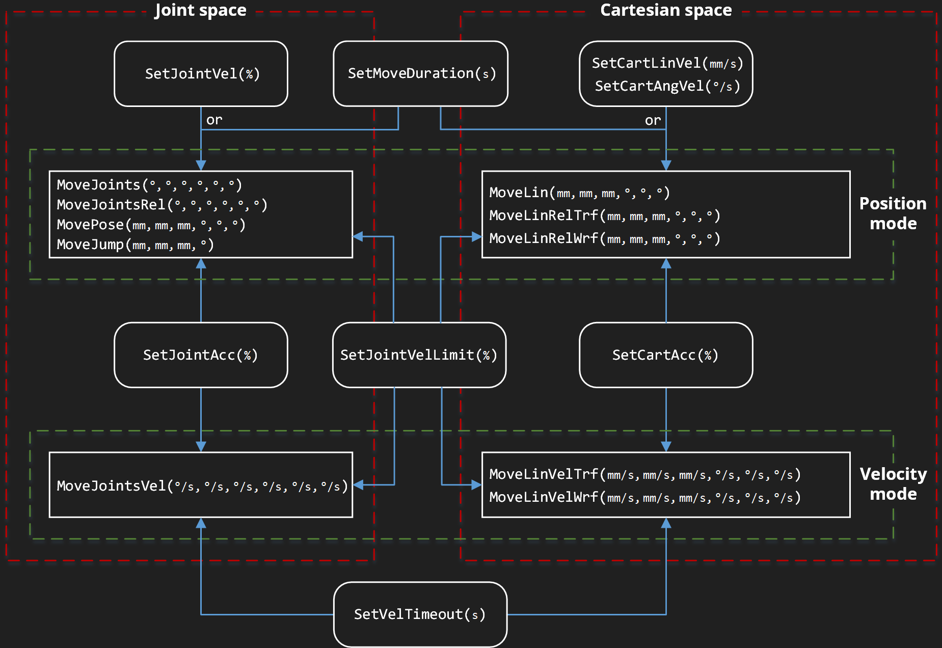
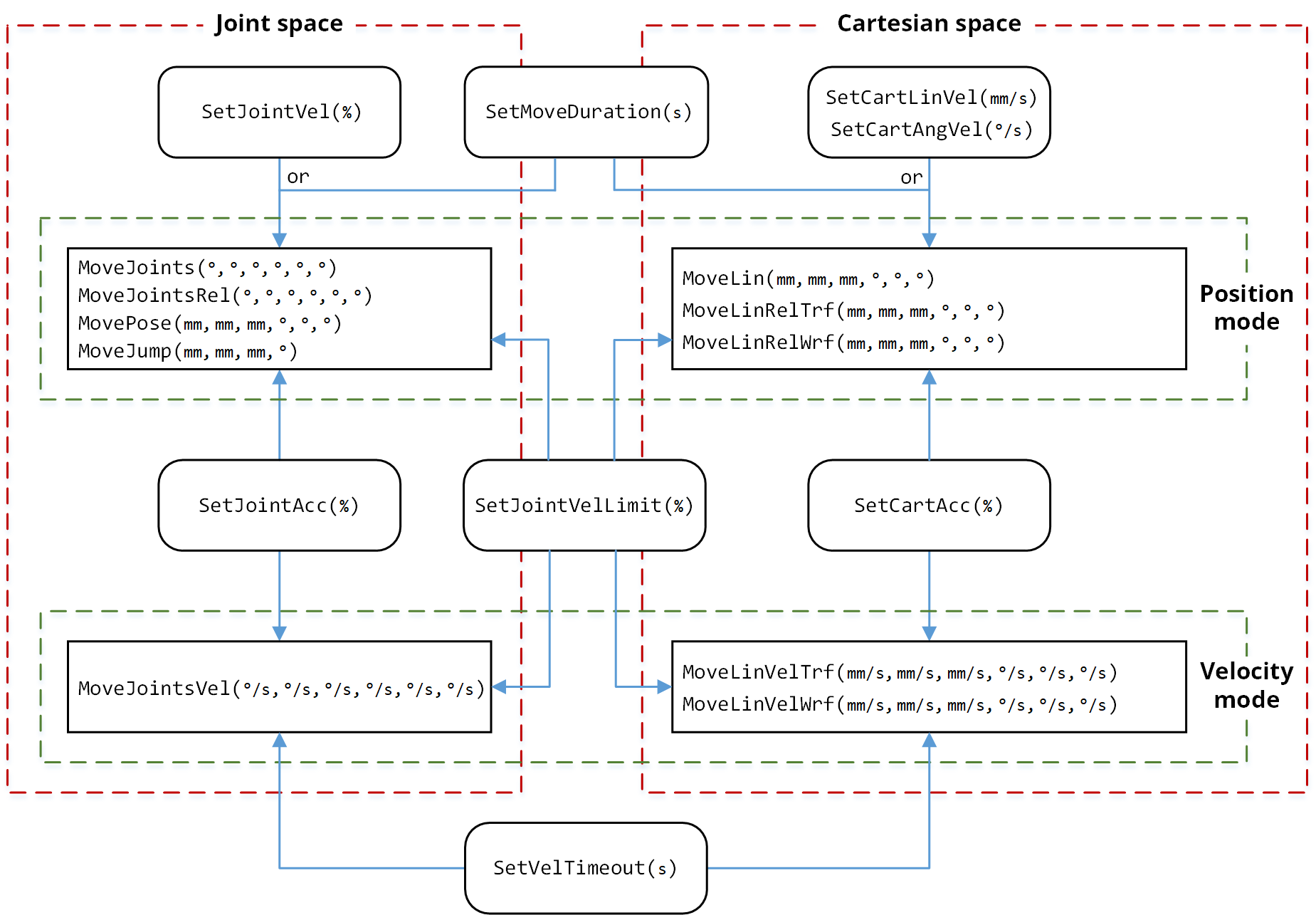
Settings that influence the robot motion in position and velocity modes

Note

The instantaneous command SetTimeScaling affects all velocities, accelerations and even time durations (including the timeout set with SetVelTimeout and the pause set with the Delay command).